利用混合磁共振成像 - 显微镜纤维束成像技术描绘结构连接组|文献速递-深度学习医疗AI最新文献

Title

题目

Imaging the structural connectome with hybrid MRI-microscopy tractography

利用混合磁共振成像 - 显微镜纤维束成像技术描绘结构连接组

01

文献速递介绍

通过多种模态绘制大脑结构能够增进我们对大脑功能、发育、衰老以及疾病的理解（汉森等人，2022；史密斯等人，2020；斯波恩斯，2013）。人们付出了很多努力，运用从磁共振成像（MRI）到显微镜成像等各种方法来创建全面的大脑连接图谱（埃森等人，2013；吴等人，2014；舍费尔等人，2020；怀特等人，2016）。然而，绘制大型大脑的全脑网络极具挑战性。不同的模态能够通过探测不同的长度尺度以及对不同的组织特征产生敏感性，提供关于潜在组织微观结构的互补信息。值得注意的是，当在同一组织中结合多种模态时，这能为多尺度神经科学带来新的机遇。 多年来，化学示踪剂一直是绘制动物大脑中神经连接通路的重要工具（贾巴迪等人，2015；莱因等人，2007；马费等人，2022；马尔科夫等人，2012）。示踪剂有助于直接可视化注射部位的轴突投射，为脑区间的连接提供高度特异性和敏感性的估计（马尔科夫等人，2012，2010）。然而，示踪剂在每只动物中仅限于单次或几次注射，要实现全脑覆盖就需要牺牲许多动物，而且综合不同个体的信息会忽略个体间重要的变异性（莱因等人，2007；马尔科夫等人，2012，2010）。此外，示踪剂禁止在人类中使用。 替代的显微镜技术是在高空间分辨率下表征纤维结构的关键参考测量方法（莫林克等人，2017）。对于在纤维束重建中有用的显微镜技术而言，显微镜必须提供三维的纤维方向信息。多种显微镜方法能够提供三维信息（例如三维偏振光成像[3D-PLI]（阿克瑟等人，2011；舒伯特等人，2017；雷克福特等人，2015）、显微计算机断层扫描（戴尔等人，2017；马西斯等人，2018）、小角X射线散射（乔治亚迪斯等人，2020）或连续电子显微镜（登克和霍斯特曼，2004）），并且在立方毫米水平上的突触结构已在人类皮质中被绘制出来（沙普森 - 科等人，2024）。然而，这些技术复杂的硬件设备和较长的采集时间限制了它们的广泛应用。因此，显微镜下的方向信息通常仅从较小的组织样本中以三维形式获取，或者从脑薄切片中以二维形式获取，这就无法在灵长类动物大脑中进行三维纤维束重建或全脑连接估计。 相比之下，扩散磁共振成像（dMRI）能够对大脑结构连接进行无创性绘制（埃德加和格里菲斯，2009）。通过测量水分子在组织中的扩散运动，我们能够推断潜在的纤维方向，并通过纤维束成像方法重建白质（WM）纤维束（博利厄，2002）。这有助于对全脑白质结构进行估计，但依赖于通过计算模型从毫米尺度的磁共振信号中估计纤维方向。模型的低分辨率和不准确会在推断的纤维方向中引入偏差或噪声，从而在下游的纤维束成像输出中导致假阳性和假阴性（迈尔 - 海因等人，2017；纳特等人，2020；席林等人，2017；托马斯等人，2014）。尽管如此，由于该方法在无创性脑连接成像方面具有巨大潜力，人们通过验证研究和方法学进展在理解和克服这些纤维束成像的局限性方面付出了大量努力（安布罗森等人，2020；艾多安和施，2018；卡米尼蒂等人，2021；科特等人，2013；德莱特等人，2019；德尔阿夸，2024；多纳休等人，2016；迪尔比等人，2007；吉拉尔等人，2020；马费等人，2022；席林等人，2019a，2019c；延迪基等人，2022；张等人，2022）。 在此，我们提出一种数据融合方法（霍华德等人，2019），联合分析来自MRI和显微镜的数据，以进行全脑的显微镜信息辅助的纤维束成像。我们的框架利用这些模态提供的互补信息来创建三维且高分辨率的混合MRI - 显微镜纤维方向（图1），在促进三维纤维束成像的同时保留显微镜成像的独特优势。我们使用二维显微镜来提供显微镜平面内纤维方向的详细估计，并使用MRI来提供跨平面的方向信息。对于后者，我们使用能够估计MRI体素内纤维方向分布的模型（贝伦斯等人，2003），而不是每个体素的单一方向（例如来自扩散张量成像的方向）（巴塞尔等人，1994）。通过从这种分布中提取与从显微镜得到的平面内方向最匹配的纤维跨平面角度，我们能够在超过MRI数据的空间分辨率下估计三维纤维方向。扩散磁共振成像的球棍（BAS）方法在每个体素中产生许多方向样本。然而，这些纤维方向在亚体素空间的精确定位是未知的。在我们的混合方法中，显微镜本质上是将三维样本的跨平面方向指定到它们在体素内的假定位置，以“超分辨”MRI信息。我们的混合MRI - 显微镜方法提供：1）三维纤维方向；2）全脑覆盖；3）高分辨率信息以及对复杂纤维结构的估计，就像显微镜所描述的那样。然后，混合方向被组合成任意分辨率的纤维方向分布（FODs），并输入到现有的纤维束成像流程中用于纤维束重建。当基于对髓鞘敏感的显微镜时，混合方向可能比MRI提供更“髓鞘特异性”的纤维方向分布，因为MRI的纤维方向分布可以代表一系列微观结构特征，包括轴突、树突和神经胶质突起（亚历山大等人，2019；杰斯珀森等人，2007；斯塔尼斯等人，1997）。这些髓鞘特异性的纤维方向分布可能在某些应用中具有优势，例如定义“髓鞘连接组”或追踪有髓纤维进入皮质。 我们使用“大麦克”数据集（霍华德等人，2023）来展示我们的方法，这是一个开放获取的多模态资源，包含来自单个猕猴大脑的死后扩散磁共振成像和显微镜数据，具有全脑覆盖。显微镜成像包括偏振光成像（PLI）（阿克瑟，2011；拉森等人，2007；舒伯特等人，2017）以及髓鞘染色（加利亚斯，1971）和尼氏染色组织学（卡达尔等人，2009；皮拉蒂等人，2008）。已经在显微镜和MRI之间进行了精确的配准，这对于在体素层面进行有意义的数据融合至关重要（胡萨尔等人，2023a）。将我们的混合方法应用于MRI和偏振光成像数据，我们首先展示如何在不同分辨率下进行混合纤维束成像，并重建跨越整个猕猴大脑的显微镜信息辅助的纤维束。在对我们的方法有信心之后，我们接着展示混合纤维束成像如何在神经解剖学和方法学研究中发挥作用。具体而言，我们利用混合输出研究基于MRI的纤维束成像中的两个已知挑战：脑回偏差（席林等人，2017）和瓶颈问题（席林等人，2022），这两个问题主要是由MRI数据有限的空间分辨率引起的。通过将我们的混合输出与同一大脑的MRI结果进行比较，我们研究这些挑战与MRI的分辨率和对比度生成机制之间的关系。然后，我们将混合纤维束成像输出与从其他动物获得的示踪剂数据进行比较（马尔科夫等人，2012，2010），以证明我们的混合方法在纤维追踪方面比仅使用MRI的纤维束成像具有更高的特异性。最后，我们使用三种不同的显微镜对比度（偏振光成像、髓鞘染色和尼氏染色组织学）进行混合纤维束成像，以展示其在不同类型显微镜上的应用。总的来说，我们的方法在不依赖侵入性示踪剂的情况下保留了显微镜成像的优势，这意味着我们能够使用一种可在包括人类在内的不同物种间转换的方法，从单个大脑中估计密集的、由显微镜信息辅助的结构连接。

Aastract

摘要

Mapping how neurons are structurally wired into whole-brain networks can be challenging, particularly in largerbrains where 3D microscopy is not available. Multi-modal datasets combining MRI and microscopy provide asolution, where high resolution but 2D microscopy can be complemented by whole-brain but lowresolution MRI.However, there lacks unified approaches to integrate and jointly analyse these multi-modal data in an insightfulway. To address this gap, we introduce a data-fusion method for hybrid MRI-microscopy fibre orientation andconnectome reconstruction. Specifically, we complement precise “in-plane” orientations from microscopy with“through-plane” information from MRI to construct 3D hybrid fibre orientations at resolutions far exceeding thatof MRI whilst preserving microscopy’s myelin specificity, resulting in superior fibre tracking. Our method isopenly available, can be deployed on standard 2D microscopy, including different microscopy contrasts, and isspecies agnostic, facilitating neuroanatomical investigation in both animal models and human brains.

绘制神经元在全脑网络中的结构连接方式颇具挑战性，尤其是在无法进行三维显微镜成像的大型脑部中。结合磁共振成像（MRI）和显微镜成像的多模态数据集提供了一种解决方案，高分辨率但二维的显微镜成像可由全脑但低分辨率的MRI成像来补充。然而，目前缺乏统一的方法来以富有洞见的方式整合和联合分析这些多模态数据。为了填补这一空白，我们引入了一种用于混合MRI - 显微镜纤维方向和连接组重建的数据融合方法。具体而言，我们用来自MRI的“跨平面”信息补充显微镜提供的精确“平面内”方向信息，以构建三维混合纤维方向，其分辨率远超MRI，同时保留显微镜成像对髓鞘的特异性，从而实现更优的纤维追踪。我们的方法是公开可用的，可应用于标准二维显微镜成像，包括不同的显微镜对比度，且不受物种限制，有助于在动物模型和人类大脑中开展神经解剖学研究。

Method

方法

2.1. MRI and microscopy data acquisition

The BigMac dataset was previously acquired and pre-processed asdescribed in Howard et al. (2023). Relevant to this work, an adult rhesusmacaque brain was scanned postmortem on a 7T small animal scanner.Structural images were acquired with multi gradient echo sequence at aspatial resolution of 0.3 mm isotropic, FOV =76.8 × 76.8 × 76.8 mm,TE/TR = 7.8/97.7 ms, and flip angle = 30◦.Postmortem dMRI was acquired with spin echo 2D multi-slicesequence and single-line readout: 0.6 mm isotropic resolution datawith 128 gradient directions at b = 4 ms/µm2 and 8 with negligibleweighting, and 1 mm isotropic resolution data with 250gradient directions at b = 4 ms/µm2 and 10 with negligible diffusionweighting.After the scanning, the brain was sectioned into two blocks (anterior/posterior halves). Each block was sectioned into thin (50/100 µm)slices and allocated to one of six interleaved contrasts: polarised lightimaging (PLI) (Axer, 2011; Axer et al., 2001, 2011; Larsen et al., 2007),Cresyl violet staining for Nissl bodies (K´ adar´ et al., 2009; Pilati et al.,2008), Gallyas silver staining for myelin (Gallyas, 1971) and threeunassigned sections that were stored for longevity. The slice thicknesswas 50 μm for 5 out of the 6 sections (including PLI, Nissl andmyelin-stained sections) with one section 100 μ**m thick. Each section ofthe same contrast was repeated every 350 µm.PLI estimated the primary fibre orientation based on the birefringence of myelinated axons with a resolution of 4 µm per pixel (Axer,2011; Axer et al., 2001, 2011; Larsen et al., 2007). Images were acquiredas the analyser (rotatable polariser) was rotated through 180◦, with a20◦ angular resolution. Images were background corrected after which asinusoid was fitted to the measured intensity at each pixel (I) as afunction of analyser rotation (ρ). The phase of the sinusoid described thein-plane fibre orientation. Retardance and transmittance maps were alsocalculated and here used only for visualisation and to drive theco-registration respectively.Histology slides with Gallyas silver staining (myelin) and Cresyl violet staining (Nissl bodies) were digitised at a spatial resolution of 0.28µm/pixel. 2D structure tensor analysis (Bigun et al., 2004; Budde andAnnese, 2013; Budde and Frank, 2012) of the stained sections (using aGaussian kernel with sigma=10 pixels) was used to estimate the fibreorientations for each microscopy pixel.

2.1. 磁共振成像（MRI）和显微镜数据采集 大麦克（BigMac）数据集先前已按照霍华德等人（Howard et al., 2023）所描述的方式进行了采集和预处理。与这项工作相关的是，一个成年恒河猴大脑在死后于7T小动物扫描仪上进行扫描。结构图像采用多梯度回波序列采集，空间分辨率为各向同性0.3毫米，视野（FOV） = 76.8×76.8×76.8毫米，回波时间（TE）/重复时间（TR） = 7.8/97.7毫秒，翻转角 = 30度。 死后扩散磁共振成像（dMRI）使用自旋回波二维多层序列和单线读出进行采集：各向同性分辨率为0.6毫米的数据，在b = 4毫秒/平方微米下有128个梯度方向，另有8个方向的权重可忽略不计；各向同性分辨率为1毫米的数据，在b = 4毫秒/平方微米下有250个梯度方向，还有10个方向的扩散权重可忽略不计。 扫描后，大脑被切成两块（前半部分/后半部分）。每一块被切成薄切片（50/100微米），并被分配到六种交错对比度中的一种：偏振光成像（PLI）（阿克瑟，2011；阿克瑟等人，2001，2011；拉森等人，2007）、用于尼氏小体的甲酚紫染色（卡达尔等人，2009；皮拉蒂等人，2008）、用于髓鞘的加利亚斯银染色（加利亚斯，1971）以及三个为长期保存而储存的未分配切片。其中五个切片（包括偏振光成像、尼氏染色和髓鞘染色切片）的切片厚度为50微米，另一个切片厚度为100微米。具有相同对比度的每个切片每隔350微米重复一次。 偏振光成像（PLI）基于有髓轴突的双折射估计主要纤维方向，分辨率为每像素4微米（阿克瑟，2011；阿克瑟等人，2001，2011；拉森等人，2007）。在分析器（可旋转偏振器）旋转180度的过程中采集图像，角度分辨率为20度。对图像进行背景校正后，将正弦曲线拟合到每个像素处测量的强度（I），作为分析器旋转（ρ）的函数。正弦曲线的相位描述了平面内的纤维方向。同时计算了相位延迟图和透射图，在此分别仅用于可视化和驱动配准。 经加利亚斯银染色（髓鞘）和甲酚紫染色（尼氏小体）的组织学切片以0.28微米/像素的空间分辨率进行数字化。对染色切片进行二维结构张量分析（比贡等人，2004；布德和安内斯，2013；布德和弗兰克，2012）（使用标准差为10像素的高斯核）来估计每个显微镜像素的纤维方向。

Results

结果

Note, we use the term MRI-microscopy to refer to the generalmethod, as multiple microscopy contrasts can be used to create hybridorientations. MRI-PLI is used to denote the hybrid orientations reconstructed using PLI which estimates the in-plane fibre orientation basedon tissue birefringence (Axer, 2011; Axer et al., 2001, 2011; Larsenet al., 2007).

需注意，我们使用“磁共振成像-显微镜成像”这一术语来指代通用方法，因为可以利用多种显微镜成像对比度来创建混合取向。“磁共振成像-偏振光成像（MRI-PLI）”用于表示通过偏振光成像（PLI）重建的混合取向，偏振光成像（PLI）是基于组织双折射来估计平面内纤维取向的（阿克瑟，2011年；阿克瑟等人，2001年、2011年；拉森等人，2007年） 。

Figure

图

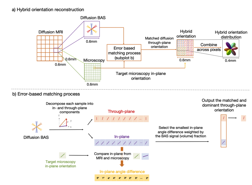
Fig. 1. The hybrid MRI-microscopy approach.a) Our data fusion method leverages the complementary strengths of diffusion MRI and microscopy. Each 2D microscopy orientation was warped to dMRI space andcompared to the BAS samples in the same voxel, where the BAS samples were first projected onto the microscopy plane to facilitate fair comparison with the 2Dmicroscopy. The microscopy through-plane information was then approximated using that from the BAS sample selected by the error-based matching process. b) Theerror based matching process. The diffusion BAS and microscopy in-plane orientation were used as inputs. The 3D BAS orientation was decomposed into the throughplane angle and in-plane angle by projecting onto the microscopy plane. The in-plane angle was compared to the target microscopy in-plane orientation byquantifying the angle difference. We selected the BAS sample with the smallest in-plane angle difference weighted by the BAS signal fraction (related to the volumefraction where more dominant fibre bundles have higher signal fractions) and determined the matched through-plane angle.

图1. 混合磁共振成像（MRI）-显微镜方法 a) 我们的数据融合方法利用了扩散磁共振成像（dMRI）和显微镜的互补优势。每个二维显微镜方向被映射到扩散磁共振成像（dMRI）空间，并与同一体素中的球棍模型（BAS）样本进行比较，其中球棍模型（BAS）样本首先被投影到显微镜平面，以便与二维显微镜进行公平比较。然后，使用基于误差匹配过程所选择的球棍模型（BAS）样本的信息来近似显微镜的跨平面信息。 b) 基于误差的匹配过程。扩散球棍模型（BAS）方向和显微镜平面内方向被用作输入。三维球棍模型（BAS）方向通过投影到显微镜平面分解为跨平面角度和平面内角度。通过量化角度差异，将平面内角度与目标显微镜平面内方向进行比较。我们选择平面内角度差异最小的球棍模型（BAS）样本，该样本由球棍模型（BAS）信号分数（与体积分数相关，更占主导地位的纤维束具有更高的信号分数）加权，并确定匹配的跨平面角度。

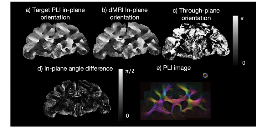
Fig. 2. The angle component used in the hybrid orientation reconstruction.a) The PLI in-plane orientation. b) The in-plane orientation from the diffusion BAS decomposition (represented by the angle of the 3D dMRI vector projected onto themicroscopy plane). Here we show the in-plane angle of the BAS sample that is most similar to the PLI. c) The through-plane orientation from the diffusion BASdecomposition (inclination angle); d) The in-plane angle difference between the target PLI orientation and the most similar BAS fibre orientation showing a smallangle difference. e) The PLI hue-saturation-value with the colour-coded orientations.

图2. 混合方向重建中使用的角度分量 a) 偏振光成像（PLI）的平面内方向。 b) 来自扩散球棍模型（BAS）分解的平面内方向（由三维扩散磁共振成像（dMRI）向量投影到显微镜平面的角度表示）。在此，我们展示与偏振光成像（PLI）最相似的球棍模型（BAS）样本的平面内角度。 c) 来自扩散球棍模型（BAS）分解的跨平面方向（倾斜角度）。 d) 目标偏振光成像（PLI）方向与最相似的球棍模型（BAS）纤维方向之间的平面内角度差，显示出较小的角度差异。 e) 带有按颜色编码方向的偏振光成像（PLI）的色调-饱和度-明度值。

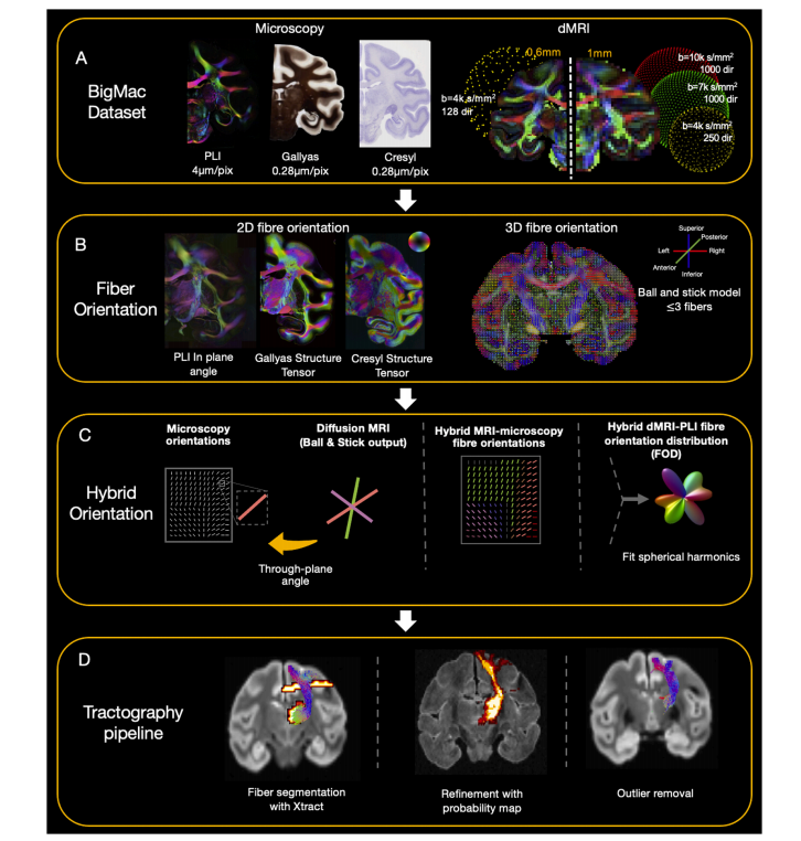
Fig. 3. An overview of the analysis pipeline.A) BigMac includes co-registered microscopy (PLI, myelin- and Nissl-staining) and postmortem MRI (dMRI/structural). B) Fibre orientations are extracted from eachmicroscopy contrast (in-plane angle from PLI, structure tensor analysis from histology) and dMRI (Ball and Stick model). C) Hybrid orientations are generated withthe in-plane orientation from microscopy and through-plane orientation from dMRI. D) The tractography results are optimised with XTRACT probability maps andoutlier removal.

图3. 分析流程概述 A) “大麦克（BigMac）”数据集包含已配准的显微镜成像数据（偏振光成像（PLI）、髓鞘染色和尼氏染色）以及死后磁共振成像数据（扩散磁共振成像（dMRI）/结构成像）。 B) 从每种显微镜成像对比度（偏振光成像的平面内角度、组织学的结构张量分析）和扩散磁共振成像（采用球棍模型）中提取纤维方向。 C) 利用显微镜成像的平面内方向和扩散磁共振成像的跨平面方向生成混合方向。 D) 利用XTRACT概率图和去除异常值来优化纤维束成像结果。

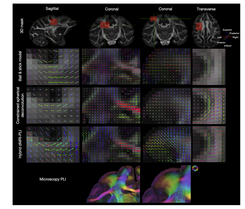
Fig. 4. Comparison between dMRI FOD and hybrid MRI-PLI FOD.The FOD generated from the Ball and Stick model (Top), constrained spherical deconvolution (Middle) and hybrid MRI-PLI (Bottom). The orientations in sagittal,coronal and transverse views are presented for U-fibres (left and right), a region covering the corpus callosum and centrum semiovale (middle left) and cortex (middleright). The PLI hue-saturation-value with the colour-coded orientations is provided at the bottom, and the contrast has been edited to highlight the grey matter. Notethe colour schemes for the FODs and PLI are not equivalent

图4. 扩散磁共振成像（dMRI）的纤维方向分布（FOD）与磁共振成像（MRI）和偏振光成像（PLI）混合的纤维方向分布（FOD）的比较 由球棍模型生成的纤维方向分布（顶部）、约束球形反卷积生成的纤维方向分布（中间）以及磁共振成像（MRI）和偏振光成像（PLI）混合生成的纤维方向分布（底部）。呈现了矢状面、冠状面和横断面视图中U形纤维（左右两侧）、涵盖胼胝体和半卵圆中心的区域（中左侧）以及皮质（中右侧）的方向。底部给出了带有按颜色编码方向的偏振光成像的色调-饱和度-明度值，并且对对比度进行了编辑以突出灰质。请注意，纤维方向分布（FOD）和偏振光成像（PLI）的配色方案并不相同。

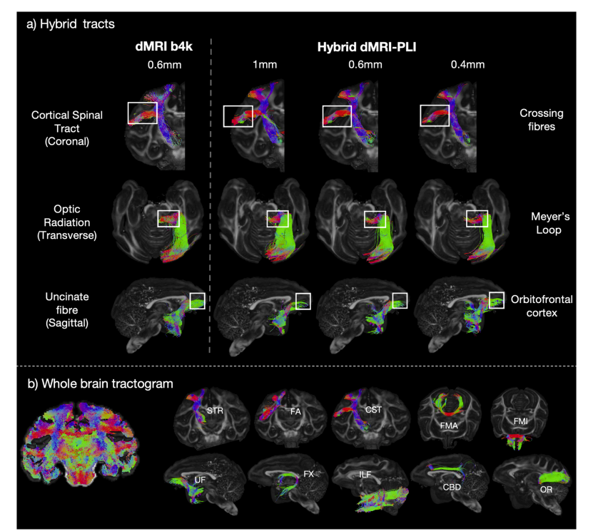
Fig. 5. Tracts generated using the hybridtractography.a) The hybrid method can successfully reconstruct tracts throughout the brain including the corticospinal tract, an example tract within the coronal plane wheremicroscopy is the most informative (Top), the optic radiation, a tract extending primarily along the anterior-posterior axis where dMRI provides most information(Middle), and the uncinate fibre (Bottom), a tract connecting the anterior temporal lobe and the orbitofrontal cortex. The anatomical features of interest are labelledwith white boxes. The background anatomical image is the fractional anisotropy behind the tracts for visualisation. b) A whole-brain tractogram is shown. Tenexample tracts generated from the hybrid tractography at 0.6 mm isotropic are illustrated including the superior thalamic radiation (STR), frontal aslant (FA),corticospinal tract (CST) in the coronal view, forceps major (FMA), forceps minor (FMI) in the axial view, uncinate fasciculus (UF), fornix (FX), inferior longitudinalfasciculus (ILF), cingulum subsection: dorsal (CBD), optic radiation (OR) in the sagittal view.

图5. 利用混合纤维束成像生成的纤维束 a) 混合方法能够成功重建全脑的纤维束，包括皮质脊髓束。冠状面内的一个纤维束示例中，显微镜成像提供了丰富的信息（上方）；视辐射，这一纤维束主要沿前后轴延伸，其中扩散磁共振成像（dMRI）提供了大部分信息（中间）；还有钩束（下方），它是连接前颞叶和眶额皮质的纤维束。感兴趣的解剖特征用白色方框标记。背景解剖图像是纤维束背后的各向异性分数，用于可视化。 b) 展示了全脑纤维束图。展示了由各向同性分辨率为0.6毫米的混合纤维束成像生成的十个示例纤维束，包括丘脑上辐射（STR）、额斜束（FA），冠状面中的皮质脊髓束（CST）、大钳（FMA）、轴面中的小钳（FMI）、钩束（UF）、穹窿（FX）、下纵束（ILF）、扣带的一个亚段：背侧扣带（CBD）、矢状面中的视辐射（OR）。

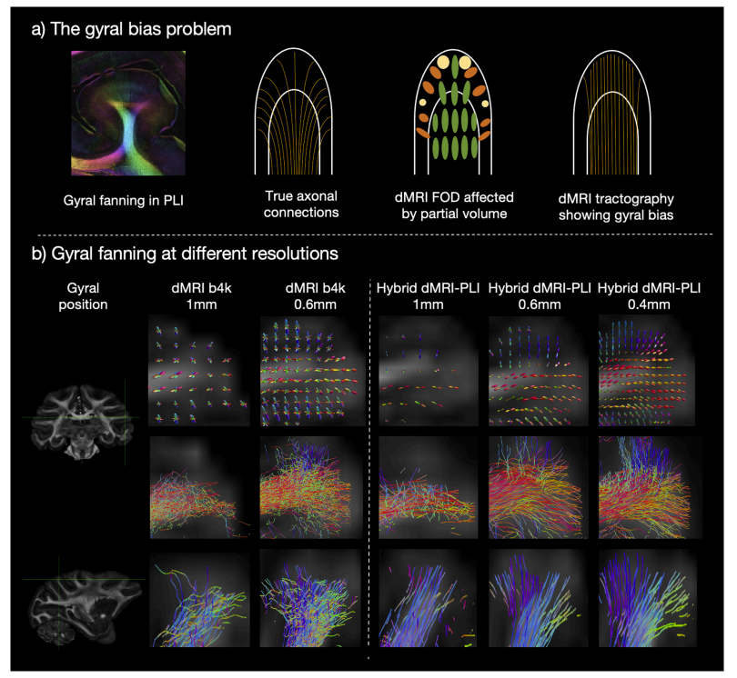
Fig. 6. High resolution hybrid tractography eliminates the gyral bias.a) Gyral bias. Diffusion tractography trajectories (streamlines) predominantly terminate at the gyral crowns but fail to turn into the gyral wall. The ground truth gyralfanning is demonstrated using PLI and a schematic representation of fibre connections. b) Gyral fanning at different resolutions. FODs (Top) and tractographystreamlines of two gyri which primarily lie within (Middle) and through (Bottom) the microscopy plane. Outputs are shown for dMRI and hybrid MRI-PLI reconstructed at different isotropic resolutions. The gyral bias problem is present in the 1 mm, whilst the high spatial resolution of 0.4 mm successfully delineates theexpected fibre fanning

图6. 高分辨率混合纤维束成像消除脑回偏差 a) 脑回偏差。扩散纤维束成像的轨迹（流线）主要终止于脑回顶部，但无法延伸至脑回壁。利用偏振光成像（PLI）以及纤维连接的示意来展示真实的脑回扇形结构。 b) 不同分辨率下的脑回扇形结构。纤维方向分布（FODs，上方）以及位于显微镜平面内（中间）和穿过显微镜平面（下方）的两个脑回的纤维束成像流线。展示了扩散磁共振成像（dMRI）以及在不同各向同性分辨率下重建的混合磁共振成像 - 偏振光成像（MRI-PLI）的结果。1毫米分辨率下存在脑回偏差问题，而0.4毫米的高空间分辨率成功描绘出预期的纤维扇形结构。

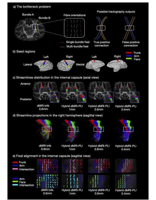
Fig. 7. Hybrid tractography preserves topography in the internal capsule.a) Bottleneck problem. An example in the internal capsule (IC) is shown (Adapted from Schilling et al., 2022). Two fibre bundles, originating and terminating atdifferent locations converge with similar orientations within the bottleneck region (truth axonal connection). Fixels (fibre orientations per voxel) are classified basedon the number of fibre bundles passing through each fixel: multi-bundle fixels (white) have multiple associated fibre bundles and single-bundle fixels have a singleassociated fibre bundle (orange). The bottleneck region, identified as the multi-bundle fixel where streamlines become indistinguishably mixed, generates falsepositive connection. As a result, a single FOD pattern can produce two probabilistic tractography outputs. b) ROIs relate to the functional representation of the trunk,arm and face regions shown for both medial and lateral parts of the two hemispheres. Tractography was seeded from the ROIs to reconstruct streamlines passingthrough the IC. c) The density map and (d) streamline projections are shown. The blue box indicates a zoomed region in (c) and the white box in (d) is the bottleneckregion of interest. The bottleneck problem is observed in the dMRI as streamlines from the ROIs are mixed. With the hybrid method, the streamlines from each ROIdemonstrate a clear anterior-posterior distribution in the bottleneck region. e) Fixel-based analysis was performed to generate a fixel density map for each ROI in theinternal capsule. The red, blue and green colours represent fixels associated with the trunk, arm and face regions respectively. Pink shows fixels associated with boththe trunk (red) and arm (blue) ROIs. Cyan shows the intersection of fixels from both the arm (blue) and face (green).

图7. 混合纤维束成像保留内囊的局部解剖特征 a) 瓶颈问题。展示了内囊（IC）的一个示例（改编自席林等人，2022）。起源和终止于不同位置的两束纤维在瓶颈区域以相似的方向汇聚（真实的轴突连接情况）。固定像素（每个体素的纤维方向，即fixel）根据穿过每个固定像素的纤维束数量进行分类：多纤维束固定像素（白色）有多个相关的纤维束，单纤维束固定像素有单个相关的纤维束（橙色）。瓶颈区域被识别为流线变得难以区分地混合的多纤维束固定像素区域，会产生假阳性连接。因此，单个纤维方向分布（FOD）模式可以产生两种概率性纤维束成像输出。 b) 感兴趣区域（ROI）与两个半球内侧和外侧部分所显示的躯干、手臂和面部区域的功能表征相关。从感兴趣区域（ROI）开始进行纤维束成像以重建穿过内囊的流线。 c) 显示了固定像素密度图，并且（d）显示了流线投影。蓝色框表示（c）中放大的区域，（d）中的白色框是感兴趣的瓶颈区域。在扩散磁共振成像（dMRI）中观察到瓶颈问题，因为来自感兴趣区域（ROI）的流线是混合的。使用混合方法时，来自每个感兴趣区域（ROI）的流线在内囊的瓶颈区域显示出清晰的前后分布。 e) 基于固定像素（fixel）的分析被用于在内囊中为每个感兴趣区域（ROI）生成固定像素密度图。红色、蓝色和绿色分别代表与躯干、手臂和面部区域相关的固定像素。粉红色表示与躯干（红色）和手臂（蓝色）感兴趣区域（ROI）都相关的固定像素。青色表示来自手臂（蓝色）和面部（绿色）的固定像素的交集部分。

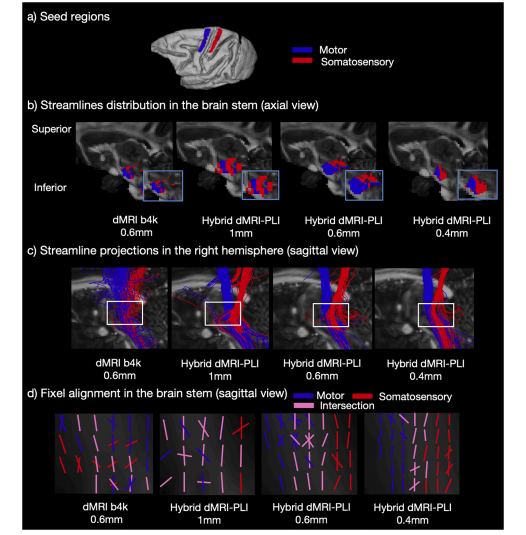
Fig. 8. Hybrid tractography preserves topography in the brainstem.a) ROIs in the primary motor (blue) and somatosensory (red) cortex. Tractography was seeded from the ROIs to reconstruct streamlines passing through thebrainstem. b) The density map in sagittal view and (c) the streamline projections are shown. The blue box indicates a zoomed region in (b) and the white box in (c) isthe bottleneck region of interest. The bottleneck problem is observed in the 0.6 mm dMRI and 1 mm hybrid method as streamlines from the two ROIs are mixed. Inthe hybrid method at higher resolution (0.6 and 0.4 mm), the streamlines from each ROI demonstrate a separable distribution in the brainstem. d) Using fixel-basedanalysis, fixels from primary motor cortex (blue), somatosensory cortex (red), and overlapping fixels (pink) are shown.

图8. 混合纤维束成像保留脑干的局部解剖特征 a) 初级运动皮层（蓝色）和躯体感觉皮层（红色）中的感兴趣区域（ROI）。从感兴趣区域（ROI）开始进行纤维束成像，以重建穿过脑干的流线。 b) 矢状面的固定像素密度图，以及（c）流线投影。蓝色框表示（b）中放大的区域，（c）中的白色框是感兴趣的瓶颈区域。在0.6毫米分辨率的扩散磁共振成像（dMRI）和1毫米分辨率的混合方法中可观察到瓶颈问题，原因是来自两个感兴趣区域（ROI）的流线混合。在更高分辨率（0.6毫米和0.4毫米）的混合方法中，来自每个感兴趣区域（ROI）的流线在脑干中呈现可分离的分布。 d) 采用基于固定像素（fixel）的分析方法，展示了来自初级运动皮层（蓝色）、躯体感觉皮层（红色）的固定像素，以及重叠的固定像素（粉红色）。

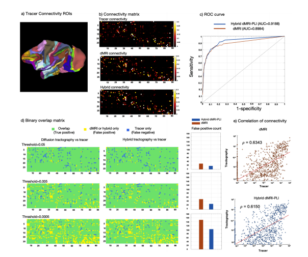
Fig. 9. Comparisons of 0.6 mm hybrid and dMRI tractography to tracer data.a) The 91 cortical areas of M132 surface parcellation are shown for the left hemisphere. b) Weighted matrices of size 29 × 91 are shown for the tracer, dMRItractography, and hybrid tractography. c) An ROC curve illustrating the specificity and sensitivity of hybrid/diffusion-only tractography relative to the tracerconnectivity. Different thresholds were applied to the tractography ranging from 0 to 0.25 and the true positive and false positive rates were calculated. d) Binaryoverlap matrices for different tractography thresholds where tracer only connections are represented in blue (false negative), tractography only in yellow (falsepositive), and overlap in green (true positive and negative). False positive connectivity was counted for dMRI and hybrid tractography. e) Scatter plot comparingtracer data with tractography (both dMRI and hybrid dMRI-PLI). Tractography data were thresholded at 1e-4 and tracer data were thresholded at 1e-6. Correlationswere investigated for several different threshold for tractography (0.0005, 0.005, 0.05), producing similar results (data not shown). The red line denotes the leastabsolute residual fit, and ρ is the Pearson correlation coefficient. Data points on the x- and y- axis (x = 0 or y = 0) were excluded from the correlation analysis.

图9. 0.6毫米混合纤维束成像、扩散磁共振成像（dMRI）纤维束成像与示踪剂数据的比较 a) 展示了左侧半球基于M132脑表面分区的91个皮质区域。 b) 示踪剂、扩散磁共振成像（dMRI）纤维束成像以及混合纤维束成像的大小为29×91的加权矩阵。 c) 受试者工作特征（ROC）曲线，说明了混合纤维束成像/仅扩散磁共振成像纤维束成像相对于示踪剂连接的特异性和敏感性。对纤维束成像应用了从0到0.25的不同阈值，并计算了真阳性率和假阳性率。 d) 不同纤维束成像阈值的二值重叠矩阵，其中仅示踪剂连接用蓝色表示（假阴性），仅纤维束成像连接用黄色表示（假阳性），重叠部分用绿色表示（真阳性和真阴性）。对扩散磁共振成像（dMRI）和混合纤维束成像统计了假阳性连接情况。 e) 示踪剂数据与纤维束成像数据（包括扩散磁共振成像（dMRI）和混合磁共振成像-偏振光成像（dMRI-PLI））的散点图。纤维束成像数据的阈值设为\(1\times10^{-4}\)，示踪剂数据的阈值设为\(1\times10^{-6}\) 。针对纤维束成像的几个不同阈值（0.0005、0.005、0.05）研究了相关性，得到了类似的结果（数据未展示）。红线表示最小绝对残差拟合，\(\rho\)是皮尔逊相关系数。坐标轴（\(x = 0\)或\(y = 0\)）上的数据点被排除在相关性分析之外。

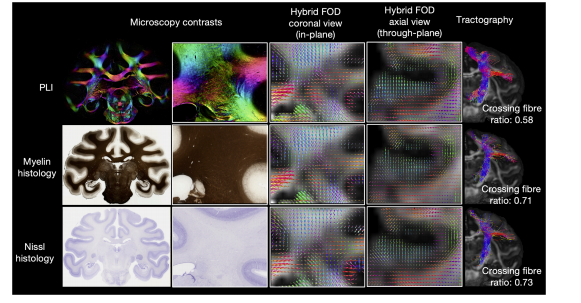
Fig. 10. Multiple microscopy contrasts can inform hybrid tractography.Hybrid fibre orientation distributions reconstructed at 0.6 mm resolution from different microscopy contrasts: PLI, myelin- and Nissl-stained histology (Gallyassilver/Cresyl violet-stained). All three contrasts show fibre orientations aligned with neuroanatomical expectations. Noticeably, the histology FODs depict moremulti-fibre voxels (crossing fibre ratio = N**wm,multi− fibre/N**wm, voxels with fibre). These FODs can be fed into tractography to reconstruct white matter tracts (examplecorticospinal tract shown).

图10. 多种显微镜成像对比度可为混合纤维束成像提供信息 从不同的显微镜成像对比度（偏振光成像（PLI）、髓鞘染色和尼氏染色组织学（加利亚斯银染色/甲酚紫染色））以0.6毫米的分辨率重建的混合纤维方向分布。这三种对比度所显示的纤维方向都符合神经解剖学预期。值得注意的是，组织学的纤维方向分布描绘出更多的多纤维体素（交叉纤维比率 = (N{wm, multi - fibre})/(N{wm, voxels with fibre})）。这些纤维方向分布可以输入到纤维束成像中，以重建白质纤维束（如图所示的皮质脊髓束的例子）。