MFCC特征提取及Griffin-Lim算法(librosa实现)
MFCC特征提取
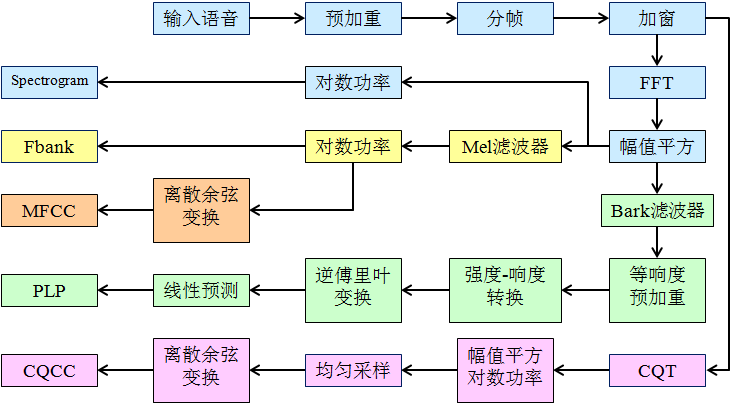
当S存在,接下来的步骤就到了离散余弦变换(DCT)步。
melspectrogram:根据名字可知mel语谱图。
power_to_db:显然就是对数功率的步骤。
def mfcc(*,y: Optional[np.ndarray] = None,sr: float = 22050,S: Optional[np.ndarray] = None,n_mfcc: int = 20,dct_type: int = 2,norm: Optional[str] = "ortho",lifter: float = 0,mel_norm: Optional[Union[Literal["slaney"], float]] = "slaney",**kwargs: Any,
) -> np.ndarray:if S is None:# multichannel behavior may be different due to relative noise floor differences between channelsS = power_to_db(melspectrogram(y=y, sr=sr, norm = mel_norm, **kwargs))fft = get_fftlib()M: np.ndarray = fft.dct(S, axis=-2, type=dct_type, norm=norm)[..., :n_mfcc, :]if lifter > 0:# shape lifter for broadcastingLI = np.sin(np.pi * np.arange(1, 1 + n_mfcc, dtype=M.dtype) / lifter)LI = util.expand_to(LI, ndim=S.ndim, axes=-2)M *= 1 + (lifter / 2) * LIreturn Melif lifter == 0:return Melse:raise ParameterError(f"MFCC lifter={lifter} must be a non-negative number")
进入melspectrogram函数可以看到S的计算过程,对应stft和幅值的平方计算。
def _spectrogram(*,y: Optional[np.ndarray] = None,S: Optional[np.ndarray] = None,n_fft: Optional[int] = 2048,hop_length: Optional[int] = 512,power: float = 1,win_length: Optional[int] = None,window: _WindowSpec = "hann",center: bool = True,pad_mode: _PadModeSTFT = "constant",
) -> Tuple[np.ndarray, int]:if S is not None:# Infer n_fft from spectrogram shape, but only if it mismatchesif n_fft is None or n_fft // 2 + 1 != S.shape[-2]:n_fft = 2 * (S.shape[-2] - 1)else:# Otherwise, compute a magnitude spectrogram from inputif n_fft is None:raise ParameterError(f"Unable to compute spectrogram with n_fft={n_fft}")if y is None:raise ParameterError("Input signal must be provided to compute a spectrogram")S = (np.abs(stft(y,n_fft=n_fft,hop_length=hop_length,win_length=win_length,center=center,window=window,pad_mode=pad_mode,))** power)return S, n_fft
Griffin-Lim 算法(vocoder)
给出声谱图,还原音频
Griffin-Lim 算法基于以下核心思想:
- 幅度谱保留:直接使用已知的幅度谱信息
- 迭代优化相位:通过迭代逐步逼近真实相位
算法流程可以概括为:
- 初始化相位(通常为随机相位)
- 通过当前相位和已知幅度谱合成复数谱
- 进行逆傅里叶变换得到时域信号
- 对时域信号进行短时傅里叶变换,提取新的相位
- 保留新相位,但使用原始已知幅度谱构建新的复数谱
- 重复步骤 3-5 直到收敛或达到最大迭代次数
import librosa
import librosa.display
import numpy as np
import soundfile as sf
import matplotlib.pyplot as plt# 1. 加载音频文件
audio_file = 'your_audio_file.wav'  # 替换为实际音频文件路径
y, sr = librosa.load(audio_file, sr=None)# 2. 提取音频特征 - 短时傅里叶变换(STFT)
n_fft = 2048
hop_length = 512
win_length = 1024D = librosa.stft(y, n_fft=n_fft, hop_length=hop_length, win_length=win_length)
S_db = librosa.amplitude_to_db(np.abs(D), ref=np.max)# 3. 可视化原始音频的频谱图
plt.figure(figsize=(10, 4))
librosa.display.specshow(S_db, sr=sr, x_axis='time', y_axis='log')
plt.colorbar(format='%+2.0f dB')
plt.title('Original Audio Spectrogram')
plt.tight_layout()
plt.savefig('original_spectrogram.png')
plt.close()# 4. 使用Griffin-Lim算法从幅度谱重建音频
n_iter = 32  # Griffin-Lim迭代次数
y_reconstructed = librosa.griffinlim(np.abs(D), n_iter=n_iter,hop_length=hop_length,win_length=win_length
)# 5. 保存重建的音频
output_file = 'reconstructed_audio.wav'
sf.write(output_file, y_reconstructed, sr)# 6. 计算原始音频和重建音频之间的均方误差(MSE)
mse = np.mean((y[:len(y_reconstructed)] - y_reconstructed) ** 2)
print(f"原始音频长度: {len(y)} 样本")
print(f"重建音频长度: {len(y_reconstructed)} 样本")
print(f"均方误差(MSE): {mse:.6f}")# 7. 可视化重建音频的频谱图
D_reconstructed = librosa.stft(y_reconstructed, n_fft=n_fft, hop_length=hop_length, win_length=win_length)
S_reconstructed_db = librosa.amplitude_to_db(np.abs(D_reconstructed), ref=np.max)plt.figure(figsize=(10, 4))
librosa.display.specshow(S_reconstructed_db, sr=sr, x_axis='time', y_axis='log')
plt.colorbar(format='%+2.0f dB')
plt.title('Reconstructed Audio Spectrogram')
plt.tight_layout()
plt.savefig('reconstructed_spectrogram.png')
plt.close()