【6.2-6.9学习周报】

提示：文章写完后，目录可以自动生成，如何生成可参考右边的帮助文档

---

摘要

本博客介绍了论文《SNNLP: Energy-Efficient Natural Language Processing Using Spiking Neural Networks》聚焦于将脉冲神经网络（SNN）应用于自然语言处理（NLP）。通过将SNN用于情感分类任务，比较不同文本编码为脉冲序列的方法。提出一种新的确定性速率编码方法，在基准NLP任务上优于常用的泊松速率编码。实验表明SNN在情感分析任务中比传统深度神经网络能效更高，虽有性能和延迟方面的小代价，但在资源受限环境有应用潜力。

Abstract

This blog introduces the paper SNNLP: Energy-Efficient Natural Language Processing Using Spiking Neural Networks, which focuses on applying Spiking Neural Networks (SNNs) to Natural Language Processing (NLP). The paper applies SNNs to sentiment classification tasks and compares different methods for encoding text into spike sequences. It introduces a novel deterministic rate coding approach that outperforms the commonly used Poisson rate coding in benchmark NLP tasks. The experiments demonstrate that SNNs achieve higher energy efficiency compared to traditional deep neural networks in sentiment analysis tasks, albeit with slight decreases in performance and increased latency, suggesting their potential for applications in resource-constrained environments.

一、模型构建方法

随着脉冲神经网络的热度不断提高，因其具有的时序性、事件驱动计算、以及低功耗等特点，越来越多的研究者将其投入到计算机视觉任务中。由于其目前在nlp任务中未取得广泛应用，因此具有不错的研究潜力可挖掘。

论文中所构建的模型主要是为了解决以下四个问题：
1)直接使用二进制嵌入还是对浮点嵌入进行速率编码，哪一种更适合NLP任务？
2）如果我们将速率编码作为一个确定性的过程而不是随机过程，我们是否会在NLP任务中看到更高的准确性？
3）在NLP任务中，我们是否看到了与之前SNN文献中报道的相同的能量-精度权衡？
4）我们能在多大程度上降低SNN的延迟成本，同时保持与传统ANN的性能竞争力？

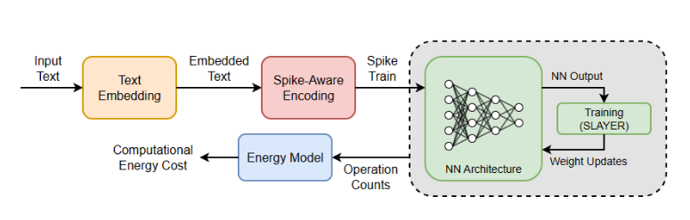
SNN和ANN的整体编码/训练管道。文本被编码为连续表示，转换为尖峰序列（用于SNN使用），并发送到下游神经网络进行训练/测试。在训练/测试期间，记录操作计数，以便我们可以计算适当的能量数字进行比较。
模型构建:研究者测试了各种编码方法，以找到正确利用网络基于时间的属性的最佳方法。也就是说，在句子和单词级别上使用以下方法-模型组合（SNN-bin除外，它只在单词级别使用）：· ANN -这是使用常规浮点嵌入的典型ANN· SNN-rate-兰德-这是在下游SNN中使用的泊松速率编码嵌入。SNN-bin -这是在下游SNN中使用的二进制嵌入。

对于研究者的比较，使用50 ms的推理窗口，SNN-bin除外，对于2类任务，SNN-bin采用512的固定长度上下文，对于6类任务，SNN-bin采用32的固定长度上下文。在这种方法中，输入文本在单词级编码并格式化为spike trains，因此需要一个非常长的上下文来表示给定输入序列中的所有单词。
研究者的自定义速率编码方法，在这项工作中称为“SNN-rate”，旨在通过修改固有的随机泊松速率编码方法（称为“SNN-rate-兰德”）来解决这个问题，从而为给定的嵌入生成确定性的尖峰序列。生成确定性编码如下：

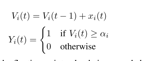
其中xi是正在编码的浮点值，Vi（t）是时间步t时神经元的膜电位，αi是神经元的膜阈值。研究者以以下方式修改了标准的Leaky Integrate-and-Fire（LIF）神经元模型：使神经元接受浮点值：selfacumulation参数、在每个时间步，仅使用存储为自累加参数的值执行累加操作，我们称之为自累加操作。

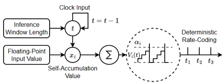
这种修改的“自累积和激发”（SAF）神经元模型仅将自累积参数xi作为输入，时钟t告诉神经元执行自累积操作多少次。此外，当神经元接收新的浮点输入时，该输入值将成为神经元的新自累积参数xi，用于所有未来的自累积操作。

然后，SAF神经元的输出被记录为速率编码尖峰序列，并直接发送到SNN的其余部分。这种修改后的“自累积和发射”（SAF）神经元，旨在提高速率编码行为的集成到SNN模型的架构，促进我们的确定性ratecoding过程。这种方法很好地适用于尖峰范例，特别是当被公式化为修改的神经元模型时。

训练方法：对于所有网络，尽可能保持其网络架构相同。所有网络都使用与所使用的嵌入技术的大小相等的输入大小。每种嵌入方法使用的输入大小如下：
·浮点和速率编码的句子嵌入：512
·浮点和速率编码的词嵌入：200
·二进制化的词嵌入：64
5个神经元用于情感分类，6个神经元用于情绪分类。
此外，SNN都使用以下神经元参数：
• threshold: 1.25
• current decay: 0.25
• voltage decay: 0.03
• tau grad: 0.03
• scale grad: 3

二、实验

1.数据集

IMDb电影评论：给定一个电影评论中的一串文本，判断文本是表达积极还是消极的情绪。

CARER:给定一条推文作为文本，决定6种情绪中的哪一种-悲伤，喜悦，爱，愤怒，恐惧或惊讶。

2.实验代码

完整实验代码链接:https://github.com/alexknipper/SNNLP

# make_graphs
# This file aims to construct the graphs used in the paper from the results
#   generated by main.py# Internal Imports# External Imports
import pandas as pd
import matplotlib
import matplotlib.pyplot as plt
from matplotlib.patches import Patch# Set library-specific globals & states
matplotlib.rcParams.update({'font.size': 18})# Globals
LOG_LOC="output/log/"
GRAPH_LOC="output/graph/final/"
colors = ["red",# red"green",# green"blue",# blue"orange",# orange"purple"# purple
]
bar_colors = [# This array contains a bunch of desaturated colors so they're easier on the eyes"#d6625c",# red"#d69b5c",# orange"#7db87a",# green"#a27db5",# purple"#5c8fd6"# blue
]
collection_names = ["sentence_imdb","sentence_emotion","word_imdb","word_emotion"
]
window_sizes = [100, 50, 25, 10]
method_collections = [["ann_sentence_imdb","snn_sentence_rate_imdb","snn_sentence_rate_rand_imdb"],["ann_sentence_emotion","snn_sentence_rate_emotion","snn_sentence_rate_rand_emotion"],["ann_word_imdb","snn_word_rate_imdb","snn_word_rate_rand_imdb","snn_word_imdb_512"],["ann_word_emotion","snn_word_rate_emotion","snn_word_rate_rand_emotion","snn_word_emotion_32"]
]# Graph 01: Plot all 100ms validation loss curves
def training_curves(name, methods, target_col="valid_loss", inference_win=50, normalize=True):# Initialize the figurefig, axs = plt.subplots(2, 2, figsize=(10,8))# Flatten the axs array for easy indexingaxs = axs.flatten()# For each collection of methods, make a graphfor (i, name, methods) in zip(range(4), collection_names, method_collections):# Start by loading in all relevant datacombined_data = pd.DataFrame()for method in methods:# Read in the log file's datafilename = (f"{LOG_LOC}final_{inference_win}ms/{method}.csv" if (method.split("_")[0] == "ann" or method.split("_")[-1].isnumeric()) else f"{LOG_LOC}final_{inference_win}ms/{method}_{inference_win}.csv")df = pd.read_csv(filename)# Add the relevant data to the combined dataframe, normalizing it if neededcombined_data[method] = (df[target_col] if not normalize else ((df[target_col] - df[target_col].min()) / (df[target_col].max() - df[target_col].min())))# Given the relevant data and appropriate labels, generate a single graphindex = 0for column_name in combined_data.columns:# Build the data labelsplit_column = column_name.split("_")label = (f"{column_name.split('_')[0]}_bin" if column_name.split("_")[-1].isnumeric() else column_name.replace(f"_{split_column[1]}", "").replace(f"_{split_column[-1]}", ""))split_label = label.split("_")label = (label.upper() if not len(split_label) > 1 else f"{split_label[0].upper()}_{'_'.join(split_label[1:])}")# Plot the dataaxs[i].plot(combined_data[column_name], label=label, color=colors[index])index += 1# Add labels and a legendaxs[i].set_xlabel("Epoch")axs[i].set_ylabel(" ".join([x.capitalize() for x in target_col.split("_")]))axs[i].legend(loc="upper right")# Adjust the layoutplt.tight_layout()# Save the plot#plt.savefig(f"{GRAPH_LOC}{methods[0][4:]}_{target_col}_curves_{inference_win}ms.jpg")plt.savefig(f"{GRAPH_LOC}{target_col}_curves_{inference_win}ms.jpg")plt.close()
#Generate all graphs
for (name, methods) in zip(collection_names, method_collections):training_curves(name, methods)# Graph 02: Plot test accuracy (as grouped bar graph) for each method on each task
#   on each inference window
def accuracy_graphs(task, measure):# Read in all performance information for all inference window sizesdata = {"imdb":{},"emotion":{}}for key in data.keys():for size in window_sizes:data[key][str(size)] = {}for size in window_sizes:# Read in the test datafilename = f"{LOG_LOC}final_{size}ms/test_results.csv"df = pd.read_csv(filename)# Store all relevant information#print(df.iloc[:,:4])for index, row in df.iloc[:,:4].iterrows():if "imdb" in row["model"]:if "ann" in row["model"]:data["imdb"]["ann"] = rowelif ("rate" in row["model"]) and (not "rate_rand" in row["model"]):data["imdb"][str(size)]["rate"] = rowelif "rate_rand" in row["model"]:data["imdb"][str(size)]["rate_rand"] = rowelse: # binarized datadata["imdb"]["bin"] = rowelse: # "emotion" in row["model"]if "ann" in row["model"]:data["emotion"]["ann"] = rowelif ("rate" in row["model"]) and (not "rate_rand" in row["model"]):data["emotion"][str(size)]["rate"] = rowelif "rate_rand" in row["model"]:data["emotion"][str(size)]["rate_rand"] = rowelse: # binarized datadata["emotion"]["bin"] = row#print(data)# Consolidate# Make graphlabels = ["ANN", "SNN-rate", "SNN-rate-rand", "SNN-bin"]fig, axs = plt.subplots(2, 1, figsize=(10,8))axs = axs.flatten()# Make the sub-graphsbar_width = .24ax_index = 0bar_index = 1for scope in ["sentence", "word"]:mod_labels = (labels if scope == "word" else labels[:-1])#print(mod_labels)for label in mod_labels:# Plot all barsif label == "ANN" or label == "SNN-bin":data_label = ("ann" if label == "ANN" else "bin")axs[ax_index].bar(bar_index, data[task][data_label][measure], bar_width/2, label=label, color=bar_colors[-1])else:data_label = ("rate" if label == "SNN-rate" else "rate_rand")i = 0for num, size in zip([0-bar_width*3/4, 0-bar_width/4, bar_width/4, bar_width*3/4], window_sizes):axs[ax_index].bar(bar_index + num, data[task][str(size)][data_label][measure], bar_width/2, label=f"{label}-{size}", color=bar_colors[i])i += 1# Set the scope to the other valuebar_index += 1# Set axis labels & constraintsif len(mod_labels) == 3:mod_labels.append("")mod_labels.insert(0, "")mod_labels.append("")#axs[ax_index].set_xlabel("Method")axs[ax_index].set_ylabel((measure.capitalize() if measure == "accuracy" else measure.upper()))axs[ax_index].set_xticks(range(len(mod_labels)))axs[ax_index].set_xticklabels(mod_labels)y_ticks = [.3, .4, .5, .6, .7, .8, .9]axs[ax_index].set_ylim(y_ticks[0], y_ticks[-1])axs[ax_index].set_yticks(y_ticks)#axs[ax_index].legend()# If this is the top graph, add the legendif scope == "sentence":# Create the legendlegend_labels = [f"{x}ms" for x in window_sizes]legend_patches = [Patch(color=bar_colors[i]) for i in range(len(legend_labels))]axs[ax_index].legend(legend_patches, legend_labels, loc="upper right")# Tweak axis valuesax_index += 1bar_index = 1# Save graphplt.savefig(f"{GRAPH_LOC}{task}_{measure}_inference_window.jpg")plt.close()
for task, measure in zip(["imdb", "emotion", "emotion"], ["accuracy", "accuracy", "mrr"]):accuracy_graphs(task, measure)

3.实验结果

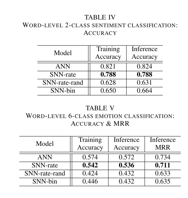
研究者观察到从ANN到其SNN对应物的预期性能下降，这是通过第VI-B节中探索的能量改进来证明的。研究者观察到泊松速率编码和二进制嵌入尖峰序列之间的类似性能，在两个任务中，二进制嵌入比典型的泊松速率编码稍微有效。·研究者观察到使用确定性编码的尖峰序列与泊松速率编码的尖峰序列相比，性能显著提高。通过扩展，也看到了使用确定性编码的尖峰序列对基于二进制嵌入的尖峰序列的类似显著改进。


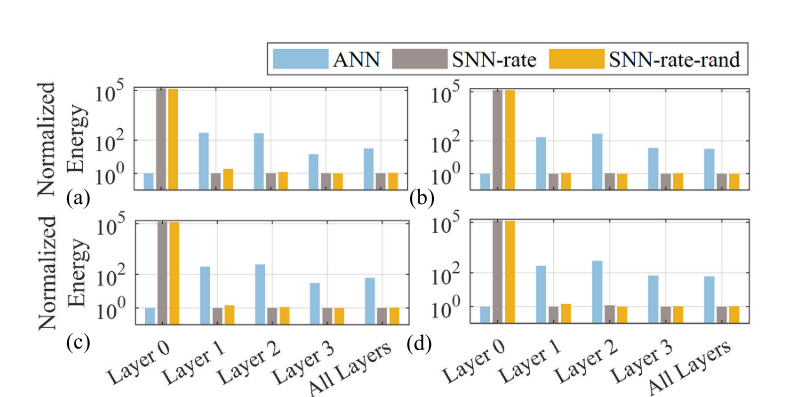
SNN在计算能量上优于ANN。在推理（a）和训练（c）期间的情感分类。推理（B）和训练（d）期间的情绪分类。

Twitter Emotion 6类情感分类任务的准确性基于推理窗口大小。上面的图描述了句子级别的性能，下面的图描述了单词级别的性能。

总结

在NLP任务中应用SNN可行且有用，尤其是资源受限环境。确定性速率编码能提高性能，缩小与ANN的差距。SNN能效高，推理和训练分别节能约32倍和60倍，同时可降低延迟。
提出新的确定性速率编码方法，在基准NLP任务上比常用的泊松速率编码准确率提高约13%，提升了SNN在NLP任务中的性能。