从头开始学习AI:第二篇 - 线性回归的数学原理与实现
回顾与引言
在上一篇中,我们实现了简单的线性回归模型。本篇将深入探讨背后的数学原理,解释代码中使用的公式,并展示如何使用scikit-learn库更高效地实现相同功能。
线性回归的数学原理
线性回归的目标是找到一条直线,使得所有数据点到这条直线的垂直距离(残差)的平方和最小。这就是所谓的最小二乘法。
1. 模型表示
简单线性回归模型可以表示为:
其中:
- y 是因变量(目标值)
- x 是自变量(特征)
- β0 是截距
- β1 是斜率
- ϵ 是误差项
2. 参数估计
我们需要找到β0和β1的最佳估计值,使得残差平方和(RSS)最小:
通过对RSS关于β0和β1求偏导并令其为零,可以得到以下解:
斜率 (β1) 的计算公式:
截距 (β0) 的计算公式:
这些公式正是我们上一篇文章中simple_linear_regression函数实现的内容。
代码实现与数学公式对应
让我们将代码与数学公式对应起来:
def simple_linear_regression(x, y):"""实现简单线性回归(一元线性回归)对应数学公式:β₁ = Σ[(xᵢ - x̄)(yᵢ - ȳ)] / Σ(xᵢ - x̄)²β₀ = ȳ - β₁x̄参数:x -- 自变量数组(特征)y -- 因变量数组(目标值)返回:slope (β₁) -- 斜率intercept (β₀) -- 截距"""# 计算均值 x̄ 和 ȳx_mean = np.mean(x) # x̄y_mean = np.mean(y) # ȳ# 计算分子 Σ[(xᵢ - x̄)(yᵢ - ȳ)]numerator = np.sum((x - x_mean) * (y - y_mean))# 计算分母 Σ(xᵢ - x̄)²denominator = np.sum((x - x_mean) ** 2)# 计算斜率 β₁slope = numerator / denominator# 计算截距 β₀ = ȳ - β₁x̄intercept = y_mean - slope * x_meanreturn slope, intercept使用scikit-learn实现
虽然自己实现算法有助于理解,但在实际项目中我们通常使用成熟的库。下面是使用scikit-learn的实现:
# 首先导入必要的库
import numpy as np
import matplotlib.pyplot as plt
from sklearn.linear_model import LinearRegression
from sklearn.metrics import mean_squared_error, r2_scoredef simple_linear_regression(x, y):"""实现简单线性回归(一元线性回归)对应数学公式:β₁ = Σ[(xᵢ - x̄)(yᵢ - ȳ)] / Σ(xᵢ - x̄)²β₀ = ȳ - β₁x̄参数:x -- 自变量数组(特征)y -- 因变量数组(目标值)返回:slope (β₁) -- 斜率intercept (β₀) -- 截距"""# 计算均值 x̄ 和 ȳx_mean = np.mean(x)  # x̄y_mean = np.mean(y)  # ȳ# 计算分子 Σ[(xᵢ - x̄)(yᵢ - ȳ)]numerator = np.sum((x - x_mean) * (y - y_mean))# 计算分母 Σ(xᵢ - x̄)²denominator = np.sum((x - x_mean) ** 2)# 计算斜率 β₁slope = numerator / denominator# 计算截距 β₀ = ȳ - β₁x̄intercept = y_mean - slope * x_meanreturn slope, interceptdef predict(x, slope, intercept):"""使用线性回归模型进行预测参数:x -- 输入值slope -- 斜率intercept -- 截距返回:预测值 y = slope * x + intercept"""return slope * x + interceptdef plot_regression(x, y, slope, intercept):"""绘制数据点和回归线参数:x -- 自变量数组y -- 因变量数组slope -- 斜率intercept -- 截距"""# 创建预测值y_pred = predict(x, slope, intercept)# 绘制散点图plt.scatter(x, y, color='blue', label='实际数据')# 绘制回归线plt.plot(x, y_pred, color='red', label='回归线')plt.xlabel('X')plt.ylabel('Y')plt.title('简单线性回归')plt.legend()plt.show()def sklearn_linear_regression(x, y):"""使用scikit-learn实现线性回归参数:x -- 自变量数组(需要reshape为二维数组)y -- 因变量数组返回:model -- 训练好的线性回归模型"""# 将x转换为二维数组 (n_samples, n_features)x_reshaped = x.reshape(-1, 1)# 创建并训练模型model = LinearRegression()model.fit(x_reshaped, y)# 输出模型参数print(f"scikit-learn实现:")print(f"斜率(系数): {model.coef_[0]:.4f}")print(f"截距: {model.intercept_:.4f}")# 计算预测值y_pred = model.predict(x_reshaped)# 计算评估指标mse = mean_squared_error(y, y_pred)r2 = r2_score(y, y_pred)print(f"均方误差(MSE): {mse:.4f}")print(f"R²分数: {r2:.4f}")return model# 示例使用
if __name__ == "__main__":# 创建示例数据np.random.seed(42)x = np.array([1, 2, 3, 4, 5, 6, 7, 8, 9, 10])y = np.array([2.1, 3.9, 6.2, 8.1, 10.2, 11.8, 14.1, 15.9, 18.2, 20.1])# 使用自定义实现slope, intercept = simple_linear_regression(x, y)print(f"\n自定义实现:")print(f"斜率: {slope:.4f}")print(f"截距: {intercept:.4f}")# 使用scikit-learn实现model = sklearn_linear_regression(x, y)# 比较两种方法的结果print("\n两种实现结果对比:")print("斜率差异:", abs(slope - model.coef_[0]))print("截距差异:", abs(intercept - model.intercept_))# 可视化结果plot_regression(x, y, slope, intercept)
自定义实现:
斜率: 2.0012
截距: 0.0533
scikit-learn实现:
斜率(系数): 2.0012
截距: 0.0533
均方误差(MSE): 0.0184
R²分数: 0.9994两种实现结果对比:
斜率差异: 0.0
截距差异: 0.0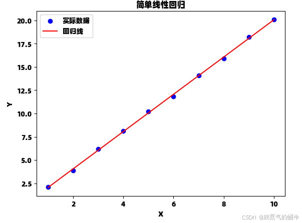
模型评估指标
在机器学习中,我们需要量化模型的性能。常用的回归评估指标有:
1. 均方误差 (MSE)
2. R²分数 (决定系数)
R²分数表示模型解释的目标变量方差的比例,取值范围在0到1之间,越接近1表示模型拟合越好。
数学推导补充
最小二乘法推导
为了找到使RSS最小的β0和β1,我们需要解以下优化问题:
对β0求偏导:
对β1求偏导:
解这组方程即可得到前面的参数估计公式。
学习心得与总结
通过本次学习,我更加深入地理解了:
- 1.线性回归背后的数学原理
- 2.最小二乘法的推导过程
- 3.如何使用scikit-learn高效实现线性回归
- 4.模型评估的重要指标
有趣的是,比较自定义实现和scikit-learn的实现结果,两者几乎完全一致(差异在浮点数精度范围内),这验证了我们自己实现的正确性。
下一步计划
- 1.学习多元线性回归及其实现
- 2.探索正则化方法(岭回归和Lasso回归)
- 3.深入研究梯度下降算法
- 4.学习交叉验证技术