VASPKIT模版INCAR笔记
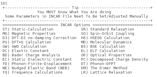
运行 vaspkit ,选择 101 菜单,可按计算类型(静态、弛豫、磁性、HSE06、GW、声子、NEB 等 20 余种)直接生成对应的 INCAR 模板。
运行 vaspkit 102 自动生成 KPOINTS,同时若目录缺少 INCAR 和 POTCAR,也会自动补齐。
生成的 INCAR 已附带注释,按需微调即可使用。
ST) Static-Calculation
静态计算
Global Parameters
ISTART = 1 (Read existing wavefunction, if there)表示如果目录中存在 WAVECAR,则从已有波函数继续计算。0:从头计算,不读取旧波函数。1:读取波函数(常用于收敛加速)。2:读取波函数和电荷密度(主要用于重启)。
ISPIN = 1 (Non-Spin polarised DFT)表示非自旋极化计算(即不考虑磁性)。1:非自旋极化(绝大多数非磁性体系)。2:自旋极化(磁性材料必须设为2)。
# ICHARG = 11 (Non-self-consistent: GGA/LDA band structures)非自洽计算(NSCF),常用于能带结构计算。11:基于静态电荷密度,只计算能带,不做电荷更新。
LREAL = .FALSE. (Projection operators: automatic)投影算符是否在实空间近似。.AUTO.:自动选择(快但不总是准确)。.FALSE.:完全在倒空间处理,最精确,推荐能带/DOS 时用。
# ENCUT = 400 (Cut-off energy for plane wave basis set, in eV)平面波截断能(单位 eV),控制基组大小。必须 ≥ POTCAR 里最大 ENMAX,建议取 1.3 × ENMAX。
# PREC = Accurate (Precision level: Normal or Accurate, set Accurate when perform structure lattice relaxation calculation)精度控制:Normal:普通精度,速度快。Accurate:高精度,推荐用于结构弛豫和能带计算。
LWAVE = .TRUE. (Write WAVECAR or not)是否写出 WAVECAR(波函数文件),通常设为 .TRUE. 方便后续继续计算。
LCHARG = .TRUE. (Write CHGCAR or not)是否写出 CHGCAR(电荷密度文件),常用于 Bader 分析、后处理。
ADDGRID= .TRUE. (Increase grid, helps GGA convergence)在 FFT 网格中加密辅助网格,改善 GGA 收敛性,推荐开启。
# LVTOT = .TRUE. (Write total electrostatic potential into LOCPOT or not)是否写出总静电势 (LOCPOT),常用于表面功函数计算。
# LVHAR = .TRUE. (Write ionic + Hartree electrostatic potential into LOCPOT or not)是否写出离子+Hartree 势(不含交换相关势)。
# NELECT = (No. of electrons: charged cells, be careful)指定体系电子数(常用于带电超胞)。需小心,否则体系总电荷不平衡。
# LPLANE = .TRUE. (Real space distribution, supercells)针对超胞的实空间分布,通常保持默认即可。
# NWRITE = 2 (Medium-level output)输出信息量:1:少量2:中等(常用)3:详细
# KPAR = 2 (Divides k-grid into separate groups)并行化参数,将 k 点分组。大体系可加速。
# NGXF = 300 (FFT grid mesh density for nice charge/potential plots)SR
# NGYF = 300 (FFT grid mesh density for nice charge/potential plots)
# NGZF = 300 (FFT grid mesh density for nice charge/potential plots)FFT 网格点数(x, y, z方向),控制电荷密度/电势的分辨率。默认由 ENCUT 决定,手动设置一般在画电荷密度时用。
Static Calculation
ISMEAR = 0 (gaussian smearing method)smearing 方法(展宽方式):0:Gaussian 展宽(常用于绝缘体/半导体)。-5:四分之一占据(tetrahedron,最精确,适合 DOS)。1, 2:金属常用(Methfessel-Paxton)。
SIGMA = 0.05 (please check the width of the smearing)smearing 宽度(单位 eV)。对绝缘体取小(0.05 eV)。对金属可大一点(0.1~0.2 eV)。
LORBIT = 11 (PAW radii for projected DOS)投影态密度 (PDOS) 设置。10:只写 DOSCAR。
11:写 DOSCAR + PROCAR,适合做投影DOS。
NEDOS = 2001 (DOSCAR points)DOSCAR 文件中的能量点数。数值越大,DOS 越平滑。
NELM = 60 (Max electronic SCF steps)SCF 最大迭代步数。一般 60 足够。
EDIFF = 1E-08 (SCF energy convergence, in eV)自洽收敛能量精度(eV)。1E-04:结构优化常用。1E-06 ~ 1E-08:高精度能带、DOS计算推荐。
SR) Standard Relaxation 标准弛豫
Global Parameters
ISTART = 1 (Read existing wavefunction, if there)
ISPIN = 1 (Non-Spin polarised DFT)
# ICHARG = 11 (Non-self-consistent: GGA/LDA band structures)
LREAL = .FALSE. (Projection operators: automatic)
# ENCUT = 400 (Cut-off energy for plane wave basis set, in eV)
# PREC = Accurate (Precision level: Normal or Accurate, set Accurate when perform structure lattice relaxation calculation)
LWAVE = .TRUE. (Write WAVECAR or not)
LCHARG = .TRUE. (Write CHGCAR or not)
ADDGRID= .TRUE. (Increase grid, helps GGA convergence)
# LVTOT = .TRUE. (Write total electrostatic potential into LOCPOT or not)
# LVHAR = .TRUE. (Write ionic + Hartree electrostatic potential into LOCPOT or not)
# NELECT = (No. of electrons: charged cells, be careful)
# LPLANE = .TRUE. (Real space distribution, supercells)
# NWRITE = 2 (Medium-level output)
# KPAR = 2 (Divides k-grid into separate groups)
# NGXF = 300 (FFT grid mesh density for nice charge/potential plots)
# NGYF = 300 (FFT grid mesh density for nice charge/potential plots)
# NGZF = 300 (FFT grid mesh density for nice charge/potential plots)
Electronic Relaxation
ISMEAR = 0 (Gaussian smearing, metals:1)
SIGMA = 0.05 (Smearing value in eV, metals:0.2)
NELM = 90 (Max electronic SCF steps)
NELMIN = 6 (Min electronic SCF steps)电子自洽最小步数,避免过早收敛。
EDIFF = 1E-08 (SCF energy convergence, in eV)电子自洽能量收敛精度。1E-04:结构优化常用。1E-06 ~ 1E-08:高精度能带/DOS 计算推荐。
# GGA = PS (PBEsol exchange-correlation)指定交换-相关泛函。PS = PBEsol,适合固体晶格常数计算。
Ionic Relaxation
NSW = 100 (Max ionic steps)离子弛豫最大步数。
IBRION = 2 (Algorithm: 0-MD, 1-Quasi-New, 2-CG)离子运动算法。0:分子动力学 (MD)。1:准牛顿法 (RMM-DIIS)。2:共轭梯度 (CG),常用于弛豫。3:快速最速下降法。
ISIF = 2 (Stress/relaxation: 2-Ions, 3-Shape/Ions/V, 4-Shape/Ions)应力和弛豫控制。2:只弛豫原子位置。3:同时弛豫原子位置 + 晶格形状 + 体积。4:弛豫原子 + 晶格形状(固定体积)。
EDIFFG = -2E-02 (Ionic convergence, eV/AA)离子收敛条件。>0:总能量变化收敛条件。<0:力收敛条件(这里是 -0.02 eV/Å,表示当最大残余力 < 0.02 eV/Å 时停止优化)。
# ISYM = 2 (Symmetry: 0=none, 2=GGA, 3=hybrids)对称性设置。0:不使用对称性。2:GGA 常用默认值。3:混合泛函(如 HSE06)时用。
LR) Lattice Relaxation
晶格弛豫
Global Parameters
ISTART = 1 (Read existing wavefunction, if there)
ISPIN = 1 (Non-Spin polarised DFT)
# ICHARG = 11 (Non-self-consistent: GGA/LDA band structures)
LREAL = .FALSE. (Projection operators: automatic)
# ENCUT = 400 (Cut-off energy for plane wave basis set, in eV)
# PREC = Accurate (Precision level: Normal or Accurate, set Accurate when perform structure lattice relaxation calculation)
LWAVE = .TRUE. (Write WAVECAR or not)
LCHARG = .TRUE. (Write CHGCAR or not)
ADDGRID= .TRUE. (Increase grid, helps GGA convergence)
# LVTOT = .TRUE. (Write total electrostatic potential into LOCPOT or not)
# LVHAR = .TRUE. (Write ionic + Hartree electrostatic potential into LOCPOT or not)
# NELECT = (No. of electrons: charged cells, be careful)
# LPLANE = .TRUE. (Real space distribution, supercells)
# NWRITE = 2 (Medium-level output)
# KPAR = 2 (Divides k-grid into separate groups)
# NGXF = 300 (FFT grid mesh density for nice charge/potential plots)
# NGYF = 300 (FFT grid mesh density for nice charge/potential plots)
# NGZF = 300 (FFT grid mesh density for nice charge/potential plots)
Lattice Relaxation
NSW = 300 (number of ionic steps)
ISMEAR = 0 (gaussian smearing method )
SIGMA = 0.05 (please check the width of the smearing)Gaussian 宽度,0.05 eV 比较小,适合非金属体系。
IBRION = 2 (Algorithm: 0-MD, 1-Quasi-New, 2-CG)
ISIF = 3 (optimize atomic coordinates and lattice parameters)
EDIFFG = -1.5E-02 (Ionic convergence, eV/A)
PREC = Accurate (Precision level)
MG) Magnetic Properties 磁性计算
Collinear Magnetic Calculation共线磁性计算
ISPIN = 2 (Spin polarised DFT)开启自旋极化计算,即考虑磁矩。1:非磁性(默认)。2:自旋极化,必须设置初始磁矩(MAGMOM)。
# MAGMOM = (Set this parameters manually)初始磁矩,必须根据原子化学价和经验给定,否则 VASP 可能收敛到非期望解。格式:MAGMOM = N*val ...例如 Fe: MAGMOM = 1*5.0 (表示 Fe 初始磁矩 5 μB)或更复杂:MAGMOM = 2*5.0 2*0.0 (两个 Fe 设 5 μB,两个 O 设 0 μB)如果不给,VASP 会默认 1 μB,可能导致收敛慢或错误解。
LASPH = .TRUE. (Non-spherical elements, d/f convergence)在 PAW 投影中考虑非球对称项,特别重要:对于 d 元素(过渡金属)和 f 元素(稀土/锕系),可以显著改善磁矩和能量收敛。对 s/p 元素影响小。
GGA_COMPAT = .FALSE. (Apply spherical cutoff on gradient field)控制梯度修正的球对称化。.TRUE.:使用旧的近似方法(更快,但对磁性可能不准)。.FALSE.:保留完整的梯度场(推荐,能更好地描述磁矩)。
VOSKOWN = 1 (Enhances the magnetic moments and the magnetic energies)使用 Vosko-Wilk-Nusair 参数化,增强磁矩和磁性能量的计算准确性。常用于磁性体系(铁磁、反铁磁)。
LMAXMIX = 4 (For d elements increase LMAXMIX to 4, f: LMAXMIX = 6)设置电荷密度混合时的球谐展开最大角动量数:2:默认,适合 s/p 元素。4:适合 d 元素(过渡金属)。6:适合 f 元素(稀土/锕系)。
# AMIX = 0.2 (Mixing parameter to control SCF convergence)电荷密度线性混合系数(默认大约 0.4)。数值越小,收敛更稳定但更慢。
# BMIX = 0.0001 (Mixing parameter to control SCF convergence)电荷密度 Broyden 混合参数(影响非线性收敛)。
# AMIX_MAG = 0.4 (Mixing parameter to control SCF convergence)磁矩部分的线性混合系数。数值小可避免磁矩震荡。
# BMIX_MAG = 0.0001 (Mixing parameter to control SCF convergence)磁矩部分的 Broyden 混合参数。
SO) Spin-Orbit Coupling
自旋轨道耦合
Spin-Orbit Coupling Calculation
LSORBIT = .TRUE. (Activate SOC)开启自旋–轨道耦合计算。必须和 ISPIN=2 一起用(体系要考虑自旋自由度)。一旦开启,计算会变成 非共线磁性 (noncollinear),磁矩可以有方向,而不仅仅是 +z 或 -z。
GGA_COMPAT = .FALSE. (Apply spherical cutoff on gradient field)在 SOC 下必须设置为 .FALSE. 才能保证正确性。
VOSKOWN = 1 (Enhances the magnetic moments and the magnetic energies)增强磁矩和磁性能量的计算精度(Vosko–Wilk–Nusair 参数化)。在 SOC 计算中依旧推荐保持开启。
LMAXMIX = 4 (For d elements increase LMAXMIX to 4, f: LMAXMIX = 6)混合电荷时的球谐展开角动量上限:4 → d 元素;6 → f 元素。SOC 对 d/f 元素影响很大,所以必须设高一点。
ISYM = -1 (Switch symmetry off)关闭对称性。SOC 计算中,晶格对称性往往会与磁矩方向冲突,必须完全关闭对称性。否则 VASP 可能强制磁矩回到高对称方向,导致结果错误。
# SAXIS = 0 0 1 (Direction of the magnetic field)定义全局磁化方向(外部磁场方向)。格式:SAXIS = x y z(单位向量)。例:0 0 1 表示 z 方向,1 0 0 表示 x 方向。
# MAGMOM = 0 0 3 (Set this parameters manually, Local magnetic moment parallel to SAXIS, 3*NIONS*1.0 for non-collinear magnetic systems)指定每个原子的初始磁矩方向和大小。在 SOC 下,必须给三分量:mx my mz。例如:MAGMOM = 0 0 3 表示磁矩初始沿 z 方向,大小约 3 μB。格式通常是 MAGMOM = N*(mx my mz),N 为原子数。注释里提到 3*NIONS*1.0,意思是如果有 N 个原子,就给 3N 个数,每个原子一个三分量。
# NBANDS = (Set this parameters manually, 2 * number of bands of collinear-run)手动设置能带数。SOC 会使能带数加倍(每个自旋态分裂)。一般取为 两倍的无 SOC 计算中 NBANDS。如果不设,VASP 会自动加倍,但可能不够,尤其在金属体系中会影响收敛。
D3) DFT-D3 no-damping Correction 色散修正
DFT-D3 Correction
IVDW = 11 (DFT-D3 method of method with no damping)IVDW = 0 → 不考虑色散相互作用(默认)。IVDW = 11 → DFT-D3 方法(Grimme D3),无阻尼 (zero damping)。IVDW = 12 → DFT-D3 方法,带 Becke-Johnson (BJ) 阻尼(通常更推荐,尤其是固体)。IVDW = 202 → DFT-D4 方法(更新版本,适合有机体系/金属有机骨架)。
PU) DFT+U Calculation DFT+U 修正
DFT+U Calculation
LDAU = .TRUE. (Activate DFT+U)开启 DFT+U 修正(在常规 DFT 基础上引入 Hubbard U 项)。主要用于 过渡金属氧化物、f 元素体系(如稀土、锕系),因为普通 GGA/LDA 对强关联系统常低估带隙、磁矩。
LDATYPE= 2 (Dudarev, only U-J matters)选择 DFT+U 的具体方法:1 → Liechtenstein 方法(U 和 J 分开,E = U − J)。2 → Dudarev 简化方法(只依赖有效 U_eff = U − J)。这里取 2 → 表示使用 Dudarev 方法,更常见更简洁。
LDAUL = 2 -1 (Orbitals for each species)指定 哪些轨道施加 U:轨道编号规则:-1=不加U, 0=s, 1=p, 2=d, 3=f。这里有两个元素:第 1 个元素 → 2 → 对 d 轨道 施加 U;第 2 个元素 → -1 → 不施加 U。
LDAUU = 2 0 (U for each species)设置每个元素的 U 值(单位 eV)。第 1 个元素 → U = 2 eV;第 2 个元素 → U = 0(即不加 U)。
LDAUJ = 0 0 (J for each species)设置每个元素的 J 值。因为 LDATYPE = 2(Dudarev),这里 J 值不会单独用到,只是形式上写上。
LMAXMIX= 4 (Mixing cut-off, 4-d, 6-f)控制电荷密度混合时的最大角动量数:对 d 元素 → 建议设为 4;对 f 元素 → 建议设为 6。否则可能导致电荷密度收敛不良。
H6) HSE06 Calculation HSE06计算(混合泛函)
HSE06 Calculation
LHFCALC= .TRUE. (Activate HF)打开 Hartree–Fock (HF) 精确交换计算。如果不开这个,计算就是普通的 GGA/PBE。
AEXX = 0.25 (25% HF exact exchange, adjusted this value to reproduce experimental band gap)设置 确切交换(Exact Exchange, EXX)所占比例。HSE06 标准取值 = 0.25 (即 25% HF 交换 + 75% GGA/PBE 交换)。这个比例可以调节:例如为了拟合实验带隙,可以略微调整。
HFSCREEN= 0.2 (Switch to screened exchange, e.g. HSE06)设定 交换作用的屏蔽参数,决定 HF 交换作用的作用范围:HFSCREEN = 0.2 → 代表 HSE06(短程 HF + 长程 PBE)。HFSCREEN = 0.0 → 代表 PBE0(全程 HF + PBE)。 HSE06 相比 PBE0 计算更快,适合周期性固体体系。
ALGO = ALL (Electronic Minimisation Algorithm, ALGO=58)指定电子结构最小化算法。ALGO = ALL 是 混合泛函计算推荐的稳定算法(内部等价于 ALGO = 58)。普通 GGA/PBE 中常用 Fast 或 Normal,但对 HF 交换不稳定,所以换用 ALL。
TIME = 0.4 (Timestep for IALGO5X)和 ALGO = ALL 相关的收敛控制参数。实际上是 IALGO = 5X 家族算法的时间步长。太大 → 不收敛,太小 → 计算效率低。
PRECFOCK= N (HF FFT grid)设置 HF 交换积分的 FFT 精度(和普通 PREC 不同):N = Norma;lF = Fast;A = Accurate;一般 Normal 就够,除非体系非常复杂(比如 f 元素、精细能带)。
# NKRED = 2 (Reduce k-grid-even only, see also NKREDX, NKREDY and NKREDZ)在 HF 计算中可 对 k 网格稀疏化,只在偶数分区下有效(如 2,4,8)。目的是减少计算量。但结果会有轻微差异,所以精度与效率需要平衡。
# HFLMAX = 4 (HF cut-off: 4d, 6f)HF 投影到的最大角动量:d 元素设 4;f 元素设 6。这类似前面 LMAXMIX 的逻辑。
# LDIAG = .TRUE. (Diagnolise Eigenvalues)是否对 HF 交换矩阵进行对角化。默认通常自动选择。如果收敛不好,可以显式设 .TRUE.。
GW) GW0 Calculation GW0计算
Global Parameters
ISTART = 1 (Read existing wavefunction, if there)
ISPIN = 1 (Non-Spin polarised DFT)
# ICHARG = 11 (Non-self-consistent: GGA/LDA band structures)
LREAL = .FALSE. (Projection operators: automatic)
# ENCUT = 400 (Cut-off energy for plane wave basis set, in eV)
# PREC = Accurate (Precision level: Normal or Accurate, set Accurate when perform structure lattice relaxation calculation)
LWAVE = .TRUE. (Write WAVECAR or not)
LCHARG = .TRUE. (Write CHGCAR or not)
ADDGRID= .TRUE. (Increase grid, helps GGA convergence)
# LVTOT = .TRUE. (Write total electrostatic potential into LOCPOT or not)
# LVHAR = .TRUE. (Write ionic + Hartree electrostatic potential into LOCPOT or not)
# NELECT = (No. of electrons: charged cells, be careful)
# LPLANE = .TRUE. (Real space distribution, supercells)
# NWRITE = 2 (Medium-level output)
# KPAR = 2 (Divides k-grid into separate groups)
# NGXF = 300 (FFT grid mesh density for nice charge/potential plots)
# NGYF = 300 (FFT grid mesh density for nice charge/potential plots)
# NGZF = 300 (FFT grid mesh density for nice charge/potential plots)
Electronic Relaxation
ISMEAR = 0
SIGMA = 0.05
EDIFF = 1E-08
step2
Electronic Relaxation
ISMEAR = 0
SIGMA = 0.05
EDIFF = 1E-08
Obtain DFT Virtual Orbitals
ALGO = EXX
LOPTICS = .TRUE.
NELM = 1
NEDOS = 2000
NBANDS = (Set this parameters manually, 50-100 per atom)
Electronic Relaxation
ISMEAR = 0
SIGMA = 0.05
EDIFF = 1E-08
step3
GW Calculation including LWANNIER90 TAG
ALGO = GW0
LSPECTRAL = .TRUE.
NOMEGA = 60
NEDOS = 2000
NELM = 1 (1-G0W0, 4-GW0)
NBANDS = (Take the same number of bands in the previous step)
# LWANNIER90 =.TRUE. (Switches on the interface between VASP and WANNIER90)
BS) BSE Calculation Bethe–Salpeter方程计算
Global Parameters
ISTART = 1 (Read existing wavefunction, if there)
ISPIN = 1 (Non-Spin polarised DFT)
# ICHARG = 11 (Non-self-consistent: GGA/LDA band structures)
LREAL = .FALSE. (Projection operators: automatic)
# ENCUT = 400 (Cut-off energy for plane wave basis set, in eV)
# PREC = Accurate (Precision level: Normal or Accurate, set Accurate when perform structure lattice relaxation calculation)
LWAVE = .TRUE. (Write WAVECAR or not)
LCHARG = .TRUE. (Write CHGCAR or not)
ADDGRID= .TRUE. (Increase grid, helps GGA convergence)
# LVTOT = .TRUE. (Write total electrostatic potential into LOCPOT or not)
# LVHAR = .TRUE. (Write ionic + Hartree electrostatic potential into LOCPOT or not)
# NELECT = (No. of electrons: charged cells, be careful)
# LPLANE = .TRUE. (Real space distribution, supercells)
# NWRITE = 2 (Medium-level output)
# KPAR = 2 (Divides k-grid into separate groups)
# NGXF = 300 (FFT grid mesh density for nice charge/potential plots)
# NGYF = 300 (FFT grid mesh density for nice charge/potential plots)
# NGZF = 300 (FFT grid mesh density for nice charge/potential plots)
Electronic Relaxation
ISMEAR = 0
SIGMA = 0.05
EDIFF = 1E-08
EL) ELF Calculation 电子局域化函数
Electron Localization Function
ISTART = 1 (Read existing wavefunction, if there)表示读取已有的 WAVECAR 文件中的波函数作为起始输入(如果存在)。对 ELF 计算来说,这样可以避免重新自洽计算,直接在收敛的波函数基础上生成 ELF 分布,更高效。
LELF = .TRUE. (Activate ELF)打开 ELF(Electron Localization Function)计算功能。
OP) Optical Properties 光学性质
Optical properties
ALGO = Exact选择 Exact Diagonalization 算法来求解电子态。在光学计算中需要高精度的本征值和波函数,因此通常不用快速近似算法,而采用精确对角化
NBANDS = (Set this parameters manually)指定计算所需的能带数(空带数量必须足够多)。
光学性质(介电函数、吸收谱等)涉及 价带 → 导带 的跃迁,因此必须设置 NBANDS 比默认更多。一般经验:至少是占据态带数的 2~3 倍,否则光学谱会截断或不准确。
LOPTICS = .TRUE.打开光学性质计算功能。VASP 会在收敛的波函数基础上计算 介电函数(ε1 和 ε2),以及由此推导的 折射率、吸收系数、能量损耗谱等。输出结果写入 OUTCAR 和 vasprun.xml,可进一步用脚本提取或用 VASPKIT 处理。
CSHIFT = 0.100给能量加一个小的虚部(单位:eV)。作用:模拟有限寿命效应,使 δ 函数峰变成 Lorentzian 展宽。避免光学谱中出现尖锐的 δ 峰。一般 0.05 ~ 0.1 eV 是常用范围。
NEDOS = 2000指定光学谱的能量分辨率(点数)。数值越大,谱线越光滑精细。2000 属于高分辨率(比通常态密度计算常用的 1000 更精细)。
ISMEAR = 0
SIGMA = 0.01
EDIFF = 1.E-8
# LPEAD = .TRUE. (Write the derivative of the cell-periodic part of the orbitals)默认关闭。打开后,VASP 会计算并输出 cell-periodic 部分轨道的导数。在某些高阶光学性质(如二阶极化率、非线性光学)计算中必须启用。常规的线性介电函数计算通常不需要。
PC) Decomposed Charge Density 分波电荷密度
Decomposed Charge Density
ISTART = 1 (Job: 0-new 1-cont 2-samecut)从已有波函数(WAVECAR)继续计算。对分解电荷计算来说,一般先做完自洽计算,再用收敛好的波函数做静态计算,因此要用 ISTART=1。
ICHARG = 1 (Read charge: 1-file 2-atom 10-const)取已有电荷密度文件(CHGCAR)。这样避免重新自洽,只做一次 非自洽(NSCF)计算 来分析态分布。
LPARD = .TRUE. (Activate decomposed charge density)激活 分解电荷密度(partial charge density) 输出功能。输出文件为 PARCHG(或分解文件 PARCHG.nk、PARCHG.nb)。
LSEPB = .TRUE. (Separately write PARCHG.nb by every band or not)是否按照 能带 band 单独输出 PARCHG.nb 文件。每个指定 band 都会生成一个文件,便于逐一分析。
LSEPK = .TRUE. (Separately write PARCHG.nk by every kpoint or not)是否按照 k 点 k-point 单独输出 PARCHG.nk 文件。每个指定 k 点都会输出对应的分解电荷文件。
Method I: Partial Charge for the specified BANDS and KPOINTS
IBAND = 20 21 22 23 (Set this parameters manually)
KPUSE = 1 2 3 4 (Set this parameters manually)
KPUSE = 1 2 3 4 (Set this parameters manually)
# Method II: Partial Charge in the energy rang of [-10.3 -5.1]
# EINT = -10.3 -5.1 (Set this parameters manually)
# EINT = -10.3 -5.1 (Set this parameters manually)
# Method III: Partial Charge in the energy rang of [EF-1 -EF]
# NBMOD=-3
# EINT = -1 (Set this parameters manually)
*********** Notes *************
(1) Copy IBZKPT as KPOINTS for static calculation,
(2) Band structure calculation.
MD) Molecular Dynamics
分子动力学
Global Parameters
ISTART = 1 (Read existing wavefunction, if there)
ISPIN = 1 (Non-Spin polarised DFT)
# ICHARG = 11 (Non-self-consistent: GGA/LDA band structures)
LREAL = .FALSE. (Projection operators: automatic)
# ENCUT = 400 (Cut-off energy for plane wave basis set, in eV)
# PREC = Accurate (Precision level: Normal or Accurate, set Accurate when perform structure lattice relaxation calculation)
LWAVE = .TRUE. (Write WAVECAR or not)
LCHARG = .TRUE. (Write CHGCAR or not)
ADDGRID= .TRUE. (Increase grid, helps GGA convergence)
# LVTOT = .TRUE. (Write total electrostatic potential into LOCPOT or not)
# LVHAR = .TRUE. (Write ionic + Hartree electrostatic potential into LOCPOT or not)
# NELECT = (No. of electrons: charged cells, be careful)
# LPLANE = .TRUE. (Real space distribution, supercells)
# NWRITE = 2 (Medium-level output)
# KPAR = 2 (Divides k-grid into separate groups)
# NGXF = 300 (FFT grid mesh density for nice charge/potential plots)
# NGYF = 300 (FFT grid mesh density for nice charge/potential plots)
# NGZF = 300 (FFT grid mesh density for nice charge/potential plots)
Electronic Relaxation
ISMEAR = 0
SIGMA = 0.05
EDIFF = 1E-08
Molecular Dynamics
IBRION = 0 (Activate MD)
NSW = 100 (Max ionic steps)
EDIFFG = -1E-02 (Ionic convergence, eV/A)
POTIM = 1 (Timestep in fs)时间步长,单位是 飞秒 (fs)。对 MD 来说,这是每一步原子运动的时间跨度。典型值 1–2 fs,太大会导致积分不稳定,太小则计算太慢。
SMASS = 0 (MD Algorithm: -3-microcanonical ensemble, 0-canonical ensemble)控制 离子温度控制算法(thermostat)。取值含义:-3 → 微正则系综 (NVE),能量守恒,不控温。0 → 正则系综 (NVT),使用 Nosé-Hoover thermostat 控温。>0 → 控温强度参数,值越大温度变化越慢。
# TEBEG = 100 (Start temperature K)初始温度,单位 K。若不指定,则使用前一步或默认值。常用于升温模拟,比如从 100 K 升到 1000 K。
# TEEND = 100 (Final temperature K)结束温度,单位 K。和 TEBEG 搭配 → 可以实现加热或冷却过程。例如 TEBEG=300, TEEND=1000 → 升温。
# MDALGO = 1 (Andersen Thermostat)控制 thermostat 算法。1 → Andersen thermostat。默认是 Nosé-Hoover thermostat。Andersen thermostat 更适合采样正则分布,但会随机扰动原子速度
# ISYM = 0 (Switch symmetry off)
NWRITE = 0 (For long MD-runs use NWRITE=0 or NWRITE=1)控制输出详细程度。对长时间 MD 计算,设为 0 或 1 可以减少输出文件大小,提高效率。
NE) Nudged Elastic Band (NEB)
NEB方法
Global Parameters
ISTART = 1 (Read existing wavefunction, if there)
ISPIN = 1 (Non-Spin polarised DFT)
# ICHARG = 11 (Non-self-consistent: GGA/LDA band structures)
LREAL = .FALSE. (Projection operators: automatic)
# ENCUT = 400 (Cut-off energy for plane wave basis set, in eV)
# PREC = Accurate (Precision level: Normal or Accurate, set Accurate when perform structure lattice relaxation calculation)
LWAVE = .TRUE. (Write WAVECAR or not)
LCHARG = .TRUE. (Write CHGCAR or not)
ADDGRID= .TRUE. (Increase grid, helps GGA convergence)
# LVTOT = .TRUE. (Write total electrostatic potential into LOCPOT or not)
# LVHAR = .TRUE. (Write ionic + Hartree electrostatic potential into LOCPOT or not)
# NELECT = (No. of electrons: charged cells, be careful)
# LPLANE = .TRUE. (Real space distribution, supercells)
# NWRITE = 2 (Medium-level output)
# KPAR = 2 (Divides k-grid into separate groups)
# NGXF = 300 (FFT grid mesh density for nice charge/potential plots)
# NGYF = 300 (FFT grid mesh density for nice charge/potential plots)
# NGZF = 300 (FFT grid mesh density for nice charge/potential plots)
Budged Elastic Band (NEB)
IMAGES = 5 (no. of images excluding two endpoints, set a NEB run no. of nodes, must be dividable by no. of images. each group of nodes works on one image. PLEASE CHANGE IT TO YOUR CHOICE NEBMAKE.PL)表示插入的 中间镜像数(不包括初末态)。实际计算中会有 IMAGES + 2 个结构(初态和末态各 1 个,中间 5 个),即一共 7 个构型。NEB 脚本(如 nebmake.pl)会根据初末态自动生成这几个镜像。
NSW = 500 (number of ionic steps)
ISMEAR = 0 (gaussian smearing method)
SIGMA = 0.05 (please check the width of the smearing)
IBRION = 3 (do MD with a zero time step)
POTIM = 0 (Zero time step so that VASP does not move the ions)
SPRING = -5.0 (spring force (eV/A2) between images)
LCLIMB = .TRUE. (turn on the climbing image algorithm)
ICHAIN = 0 (Indicates which method to run. NEB (ICHAIN=0) is the default)
IOPT = 1 (LBFGS = Limited-memory Broyden-Fletcher-Goldfarb-Shanno)控制优化算法。1 → LBFGS (Limited-memory Broyden-Fletcher-Goldfarb-Shanno),是一种拟牛顿法,适合 NEB 路径优化。其他常见取值:2 → Conjugate Gradient (CG)。3 → Quick-Min。
DM) Dimer Method
二聚体方法(过渡态搜索)
Global Parameters
ISTART = 1 (Read existing wavefunction, if there)
ISPIN = 1 (Non-Spin polarised DFT)
# ICHARG = 11 (Non-self-consistent: GGA/LDA band structures)
LREAL = .FALSE. (Projection operators: automatic)
# ENCUT = 400 (Cut-off energy for plane wave basis set, in eV)
# PREC = Accurate (Precision level: Normal or Accurate, set Accurate when perform structure lattice relaxation calculation)
LWAVE = .TRUE. (Write WAVECAR or not)
LCHARG = .TRUE. (Write CHGCAR or not)
ADDGRID= .TRUE. (Increase grid, helps GGA convergence)
# LVTOT = .TRUE. (Write total electrostatic potential into LOCPOT or not)
# LVHAR = .TRUE. (Write ionic + Hartree electrostatic potential into LOCPOT or not)
# NELECT = (No. of electrons: charged cells, be careful)
# LPLANE = .TRUE. (Real space distribution, supercells)
# NWRITE = 2 (Medium-level output)
# KPAR = 2 (Divides k-grid into separate groups)
# NGXF = 300 (FFT grid mesh density for nice charge/potential plots)
# NGYF = 300 (FFT grid mesh density for nice charge/potential plots)
# NGZF = 300 (FFT grid mesh density for nice charge/potential plots)
The dimer method
NSW = 500 (number of ionic steps)
ISMEAR = 0 (gaussian smearing method )
SIGMA = 0.05 (please check the width of the smearing)
IBRION = 3 (do MD with a zero time step)
POTIM = 0 (Zero time step so that VASP does not move the ions)
ICHAIN = 2 (Use the dimer method required for the latest code)
DdR = 0.005 (The dimer separation, twice the distance between images)dimer 分离距离,单位 Å。实际上就是两个“像”之间的间隔(dimer = 2 个结构)。设置过大会影响精度,过小会增加噪声。0.005 Å 是常见合理值。
DRotMax = 1 (Maximum number of rotation steps per translation step)每个平移步骤中允许的 最大旋转步数。dimer 在搜索过程中会不断旋转以找到不稳定方向。值太小可能导致方向没找准,太大则计算量增加。
DFNMin = 0.01 (Magnitude of the rotational force below which the dimer is not rotated)旋转力阈值(下限)。当旋转力小于该值时,不再旋转 dimer,认为已经找到主导不稳定模式。
DFNMax = 1.0 (Magnitude of the rotational force below which dimer rotation stops)旋转力阈值(上限)。当旋转力大于该值时,旋转停止(避免过度迭代)。
IOPT = 2 (CG = Conjugate Gradient)
FQ) Frequency Calculations
振动频率计算
Global Parameters
ISTART = 1 (Read existing wavefunction, if there)
ISPIN = 1 (Non-Spin polarised DFT)
# ICHARG = 11 (Non-self-consistent: GGA/LDA band structures)
LREAL = .FALSE. (Projection operators: automatic)
# ENCUT = 400 (Cut-off energy for plane wave basis set, in eV)
# PREC = Accurate (Precision level: Normal or Accurate, set Accurate when perform structure lattice relaxation calculation)
LWAVE = .TRUE. (Write WAVECAR or not)
LCHARG = .TRUE. (Write CHGCAR or not)
ADDGRID= .TRUE. (Increase grid, helps GGA convergence)
# LVTOT = .TRUE. (Write total electrostatic potential into LOCPOT or not)
# LVHAR = .TRUE. (Write ionic + Hartree electrostatic potential into LOCPOT or not)
# NELECT = (No. of electrons: charged cells, be careful)
# LPLANE = .TRUE. (Real space distribution, supercells)
# NWRITE = 2 (Medium-level output)
# KPAR = 2 (Divides k-grid into separate groups)
# NGXF = 300 (FFT grid mesh density for nice charge/potential plots)
# NGYF = 300 (FFT grid mesh density for nice charge/potential plots)
# NGZF = 300 (FFT grid mesh density for nice charge/potential plots)
Frequence Calculations
NSW = 1 (number of ionic steps. Make it odd.)
ISMEAR = 0 (gaussian smearing method)
SIGMA = 0.05 (please check the width of the smearing)
IBRION = 5 (frequence calculation)
POTIM = 0.02 (displacement step)
DC) Elastic Constant
弹性常数
Global Parameters
ISTART = 1 (Read existing wavefunction, if there)
ISPIN = 1 (Non-Spin polarised DFT)
# ICHARG = 11 (Non-self-consistent: GGA/LDA band structures)
LREAL = .FALSE. (Projection operators: automatic)
# ENCUT = 400 (Cut-off energy for plane wave basis set, in eV)
# PREC = Accurate (Precision level: Normal or Accurate, set Accurate when perform structure lattice relaxation calculation)
LWAVE = .TRUE. (Write WAVECAR or not)
LCHARG = .TRUE. (Write CHGCAR or not)
ADDGRID= .TRUE. (Increase grid, helps GGA convergence)
# LVTOT = .TRUE. (Write total electrostatic potential into LOCPOT or not)
# LVHAR = .TRUE. (Write ionic + Hartree electrostatic potential into LOCPOT or not)
# NELECT = (No. of electrons: charged cells, be careful)
# LPLANE = .TRUE. (Real space distribution, supercells)
# NWRITE = 2 (Medium-level output)
# KPAR = 2 (Divides k-grid into separate groups)
# NGXF = 300 (FFT grid mesh density for nice charge/potential plots)
# NGYF = 300 (FFT grid mesh density for nice charge/potential plots)
# NGZF = 300 (FFT grid mesh density for nice charge/potential plots)
Elastic constants Calculation
# NGZF = 300 (FFT grid mesh density for nice charge/potential plots)
IBRION = 6 (Determine the Hessian matrix)
NFREE = 2 (How many displacements are used for each direction, 2-4)
ISIF = 3 (Stress/relaxation: 3-Shape/Ions/V)
NSW = 1 (Max ionic steps)
PREC = High (High level)
# ENCUT = 700 (1.3 ~ 1.5 * default cutoff, need to check convergence)
BD) Bader Charge Analysis Bader 电荷分析
Bader Charge Analysis
LAECHG = .TRUE. (Write core charge into CHGCAR file)
LCHARG = .TRUE. (Write CHGCAR file)
(主要依赖 CHGCAR 输出,用 bader 程序分析,INCAR 无特殊要求)
EC) Static Dielectric Constant
静态介电常数
Global Parameters
ISTART = 1 (Read existing wavefunction, if there)
ISPIN = 1 (Non-Spin polarised DFT)
# ICHARG = 11 (Non-self-consistent: GGA/LDA band structures)
LREAL = .FALSE. (Projection operators: automatic)
# ENCUT = 400 (Cut-off energy for plane wave basis set, in eV)
# PREC = Accurate (Precision level: Normal or Accurate, set Accurate when perform structure lattice relaxation calculation)
LWAVE = .TRUE. (Write WAVECAR or not)
LCHARG = .TRUE. (Write CHGCAR or not)
ADDGRID= .TRUE. (Increase grid, helps GGA convergence)
# LVTOT = .TRUE. (Write total electrostatic potential into LOCPOT or not)
# LVHAR = .TRUE. (Write ionic + Hartree electrostatic potential into LOCPOT or not)
# NELECT = (No. of electrons: charged cells, be careful)
# LPLANE = .TRUE. (Real space distribution, supercells)
# NWRITE = 2 (Medium-level output)
# KPAR = 2 (Divides k-grid into separate groups)
# NGXF = 300 (FFT grid mesh density for nice charge/potential plots)
# NGYF = 300 (FFT grid mesh density for nice charge/potential plots)
# NGZF = 300 (FFT grid mesh density for nice charge/potential plots)
Electronic Relaxation
ISMEAR = 0
SIGMA = 0.05
EDIFF = 1E-08
LEPSILON = .TRUE. (Determined by density functional perturbation theory)
# LCALCEPS = .TRUE. (OR Determined by self-consistent response of the system to a finite electric field)
LPEAD = .TRUE. (Determined derivative of the cell-periodic part of the orbitals using finite differences)
FD) Phonon-Finite-Displacement
声子有限位移法
ISMEAR = 0 (Gaussian smearing)
SIGMA = 0.01 (Smearing value in eV)
IBRION = -1 (Ions are not moved)
EDIFF = 1E-08 (SCF energy convergence, in eV)
PREC = Accurate (Precision level)
# ENCUT = 500 (Cut-off energy for plane wave basis set, in eV)
IALGO = 38 (Davidson block iteration scheme)
LREAL = .FALSE. (Projection operators: false)
LWAVE = .FLASE. (Write WAVECAR or not)
LCHARG = .FLASE. (Write CHGCAR or not)
ADDGRID= .TRUE. (Increase grid, helps GGA convergence)
DT) Phonon-DFPT 声子密度泛函微扰理论
ISMEAR = 0 (Gaussian smearing)
SIGMA = 0.05 (Smearing value in eV)
IBRION = 8 (determines the Hessian matrix using DFPT)
EDIFF = 1E-08 (SCF energy convergence, in eV)
PREC = Accurate (Precision level)
# ENCUT = 500 (Cut-off energy for plane wave basis set, in eV)
IALGO = 38 (Davidson block iteration scheme)
LREAL = .FALSE. (Projection operators: false)
LWAVE = .FLASE. (Write WAVECAR or not)
LCHARG = .FLASE. (Write CHGCAR or not)
ADDGRID= .TRUE. (Increase grid, helps GGA convergence)