去噪扩散概率模型（DDPM）全解：从数学基础到实现细节

一、 概述

在这篇博客文章中，我们将深入探讨去噪扩散概率模型（也被称为 DDPMs，扩散模型，基于得分的生成模型，或简称为自动编码器），这可以说是AIGC最近几年飞速发展的基石，如果你想做生成式人工智能，这个模型肯定是绕不过的门槛，基于扩散模型，研究人员已经在图像/音频/视频的有条件或无条件生成任务中取得了显著成果。当前一些流行的应用包括 OpenAI 的 GLIDE 和 DALL-E 2，海德堡大学的 Latent Diffusion，以及 Google Brain 的 ImageGen。

这篇文章详细介绍 (Ho 等人，2020) 提出的原始 DDPM 论文公式推导过程，并基于 Phil Wang 的 PyTorch 实现（其本身基于 原始 TensorFlow 实现）进行逐步实现。需要注意的是，用扩散方法进行生成建模的想法最早其实是在 (Sohl-Dickstein 等人，2015) 中提出的。然而，直到 (Song 等人，2019)（斯坦福大学）和随后 (Ho 等人，2020)（Google Brain）分别改进该方法之后，它才真正引起广泛关注。

• 公式推导本文学习的是：龙老师教AI的Diffusion Model | 扩散模型原理及代码实现，3小时快速上手
• 代码GitHub地址：https://github.com/huggingface/notebooks/blob/main/examples/annotated_diffusion.ipynb

其他生成模型如GAN、Normalizing Flows相比，扩散模型其实并不复杂：它们的共同点都是从一个简单分布中的噪声出发，转换为真实的数据样本。在扩散模型中，神经网络学习逐步对数据去噪，从纯噪声开始恢复出图像

二、论文解读

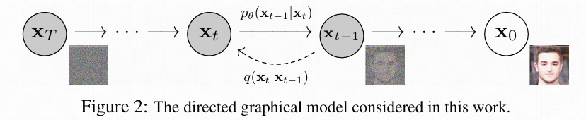
对于生成图像来说，可以分为两个阶段：

1. 前向扩散过程：逐步向图像添加高斯噪声，直到最终变成纯噪声

目标：得到每个时间步t的加噪图像

引入两个参数 ${\alpha }_t$和 ${\beta }_t$, 其中 ${\alpha }_t$=1-${\beta }_t$

$${\alpha }_t=1-{\beta }_t$$ $\beta$ 越来越大，论文中0.0001到0.002,从而 $\alpha$ 也就是要越来越小（噪声需要随步数增多）
$$x_t=\sqrt{a_t}{x}_{t-1}+\sqrt{1-{\alpha }_t}{z}_1$$
$z_t$是由标准正太分布采样得到的噪声,对应代码就是：

x = torch.randn(batch_size, channels, height, width)

需要得到 $x_t$由$x_0$直接得到的公式，这和训练过程有关，在每个训练步骤中，对于一个 batch，每张图片只随机选取一个时间步 t，然后训练模型去预测该时间步下的噪声。推到过程如下：

$x_{t-1}=\sqrt{a_{t-1}}{x}_{t-2}+\sqrt{1-{\alpha }_{t-1}}{z}_2$ 带入到上式得：

$$x_t=\sqrt{a_t}(\sqrt{a_{t-1}}{x}_{t-2}+\sqrt{1-{\alpha }_{t-1}}{z}_2)+\sqrt{1-{\alpha }_t}{z}_1$$

其中每次加入的噪声都服从高斯分布$z_1,z_2,\dots \sim \mathcal{N}(0,1)$，化简得：

$$x_t=\sqrt{a_t{a}_{t-1}}{x}_{t-2}+(\sqrt{a_t(1-{\alpha }_{t-1})}{z}_2+\sqrt{1-{\alpha }_t}{z}_1)$$

括号两项里分别服从 $\mathcal{N}(0,1-{\alpha }_t)$，$\mathcal{N}(0,a_t(1-{\alpha }_{t-1}))$

这里就是相加后仍服从高斯分布，即$\sqrt{a_t(1-{\alpha }_{t-1})}{z}_2+\sqrt{1-{\alpha }_t}{z}_1\sim \mathcal{N}(0,(1-{\alpha }_t{\alpha }_{t-1}))$，得到：
$$x_t=\sqrt{{\alpha }_t{\alpha }_{t-1}}{x}_{t-2}+\sqrt{1-{\alpha }_t{\alpha }_{t-1}}{z}_2$$不断往里套, 就能发现规律了, 其实就是累乘:
$$x_t=\sqrt{{\overline{\alpha }}_t}{x}_0+\sqrt{1-{\overline{\alpha }}_t}{z}_t$$
可以看到$x_t$其实可以看成是原始数据 $x_0$和随机噪音$z_t$的线性组合，其中$\sqrt{{\overline{\alpha }}_t}$和$\sqrt{1-{\overline{\alpha }}_t}$为组合系数，它们的平方和等于1

2. 反向去噪过程

目标:就是通过一个纯噪声图像一步步去噪还原为特定分布的图像（正常图像），其中神经网络被训练用于预测噪声

一步一步来，要求$q\left(x_{t-1}|x_t\right)$很麻烦，但如果引入$x_0$作为已知量，利用贝叶斯公式就可以得到下式：
$$q\left(x_{t-1}|x_t,x_0\right)=q\left(x_t|x_{t-1},x_0\right)\frac{q\left(x_{t-1}|x_0\right)}{q\left(x_t|x_0\right)}$$

已知$x_0$的情况下，各个因式都能够求出来并且符合正太分布：
$$q\left({\mathbf{x}}_{t-1}|{\mathbf{x}}_0\right)=\sqrt{{\overline{a}}_{t-1}}{\mathbf{x}}_0+\sqrt{1-{\overline{a}}_{t-1}}\mathbf{z}\sim \mathcal{N}\left(\sqrt{{\overline{a}}_{t-1}}{\mathbf{x}}_0,1-{\overline{a}}_{t-1}\right)$$
$$q\left({\mathbf{x}}_t|{\mathbf{x}}_0\right)=\sqrt{{\overline{a}}_t}{\mathbf{x}}_0+\sqrt{1-{\overline{a}}_t}\mathbf{z}\sim \mathcal{N}\left(\sqrt{{\overline{a}}_t}{\mathbf{x}}_0,1-{\overline{a}}_t\right)$$
$$q\left({\mathbf{x}}_t|{\mathbf{x}}_{t-1},{\mathbf{x}}_0\right)=\sqrt{a_t}{\mathbf{x}}_{t-1}+\sqrt{1-{\mathbf{\alpha }}_t}\mathbf{z}\sim \mathcal{N}\left(\sqrt{a_t}{\mathbf{x}}_{t-1},\begin{array}{c}1-{\mathbf{\alpha }}_t\end{array}\right)$$

将正太分布转换为e的指数形式进行乘除运算：

连续型随机变量 X 如果有如下形式的密度函数： $$f\left(x\right)=\frac{1}{\sqrt{2\pi }\sigma }{e}^{-\frac{{\left(x-\mu \right)}^2}{2{\sigma }^2}}\left(\mu \in R,\sigma >0\right)$$
则称 X 服从参数为$(\mu ,{\sigma }^2)$ 的正态分布(normaldistribution) ,记为 $X-N(\mu ,{\sigma }^2)$

得到结果：
$$\propto \exp (-\frac{1}{2}(\frac{({\mathbf{x}}_t-\sqrt{{\alpha }_t}{\mathbf{x}}_{t-1}{)}^2}{{\beta }_t}+\frac{({\mathbf{x}}_{t-1}-\sqrt{{\bar{\alpha }}_{t-1}}{\mathbf{x}}_0{)}^2}{1-{\bar{\alpha }}_{t-1}}-\frac{({\mathbf{x}}_t-\sqrt{{\bar{\alpha }}_t}{\mathbf{x}}_0{)}^2}{1-{\bar{\alpha }}_t}\left)\right)$$

将平方项展开，合并同类项：

$$\begin{array}{c}\propto \exp \left(-\frac{1}{2}\left(\frac{({\mathbf{x}}_t-\sqrt{{\alpha }_t}{\mathbf{x}}_{t-1}{)}^2}{{\beta }_t}+\frac{({\mathbf{x}}_{t-1}-\sqrt{{\bar{\alpha }}_{t-1}}{\mathbf{x}}_0{)}^2}{1-{\bar{\alpha }}_{t-1}}-\frac{({\mathbf{x}}_t-\sqrt{{\bar{\alpha }}_t}{\mathbf{x}}_0{)}^2}{1-{\bar{\alpha }}_t}\right)\right)\\ =\exp \left(-\frac{1}{2}(\frac{{\mathbf{x}}_t^2-2\sqrt{{\alpha }_t}{\mathbf{x}}_t{\mathbf{x}}_{t-1}+{\alpha }_t{\mathbf{x}}_{t-1}^2}{{\beta }_t}+\frac{{\mathbf{x}}_{t-1}^2-2\sqrt{{\bar{\alpha }}_{t-1}}{\mathbf{x}}_0{\mathbf{x}}_{t-1}+{\bar{\alpha }}_{t-1}{\mathbf{x}}_0^2}{1-{\bar{\alpha }}_{t-1}}-\frac{({\mathbf{x}}_t-\sqrt{{\bar{\alpha }}_t}{\mathbf{x}}_0{)}^2}{1-{\bar{\alpha }}_t})\right)\\ =\exp \left(-\frac{1}{2}\left((\frac{{\alpha }_t}{{\beta }_t}+\frac{1}{1-{\bar{\alpha }}_{t-1}}){\mathbf{x}}_{t-1}^2-(\frac{2\sqrt{{\alpha }_t}}{{\beta }_t}{\mathbf{x}}_t+\frac{2\sqrt{{\bar{\alpha }}_{t-1}}}{1-{\bar{\alpha }}_{t-1}}{\mathbf{x}}_0){\mathbf{x}}_{t-1}+C({\mathbf{x}}_t,{\mathbf{x}}_0)\right)\right)\end{array}$$

$\exp \left(-\frac{{\left(x-\mu \right)}^2}{2{\sigma }^2}\right)=\exp \left(-\frac{1}{2}\left(\frac{1}{{\sigma }^2}{x}^2-\frac{2\mu }{{\sigma }^2}x+\frac{{\mu }^2}{{\sigma }^2}\right)\right)$

因为是要得到$x_{t-1}$的分布，所以将其他看作常熟进行化简，得到得结果和标准正太分布比对，即可得到均值和方差，也就能得到$x_{t-1}$的分布，分析上式可以知道方差是个常数，仅和${\alpha }_t$、${\beta }_t$有关（这是提前设好的值）:
$$\begin{array}{rl}{\sigma }^2& =1/(\frac{{\alpha }_t}{{\beta }_t}+\frac{1}{1-\overline{{\alpha }_{t-1}}})\\ & =1/(\frac{{\alpha }_t-{\alpha }_t\ast \overline{{\alpha }_{t-1}}+{\beta }_t}{{\beta }_t\ast (1-\overline{{\alpha }_{t-1}})})\\ & =\frac{1-\overline{{\alpha }_{t-1}}}{1-\overline{{\alpha }_t}}\ast {\beta }_t\end{array}$$

可以得到均值：
$${\tilde{\mu }}_{t-1}\left(x_t,x_0\right)=\frac{\sqrt{{\alpha }_t}\left(1-{\overline{\alpha }}_{t-1}\right)}{1-{\overline{\alpha }}_t}{x}_t+\frac{\sqrt{{\overline{\alpha }}_{t-1}}{\beta }_t}{1-{\overline{\alpha }}_t}{x}_0$$

可以看出只和$x_t,x_0$有关系，而$x_0$是我们要求得目标是不知道的，可以根据第一个得到的公式：
$$x_t=\sqrt{{\overline{\alpha }}_t}{x}_0+\sqrt{1-{\overline{\alpha }}_t}{z}_t$$

可以得到：
$$x_0=\frac{1}{\sqrt{{\alpha }_t}}\left(x_t-\sqrt{1-{\overline{\alpha }}_t}{z}_t\right)$$

Tips:既然已知$x_0$和$x_t$的关系，为什么不直接一步求解？

扩散模型包括两个过程：前向过程（forward process）和反向过程（reverse process），其中前向过程又称为扩散过程（diffusion process），无论是前向过程还是反向过程都是一个参数化的马尔可夫链（Markov chain）

马尔可夫链是指一个随机过程，其中系统状态的未来演变仅依赖于当前状态，而与过去的状态无关。

将 $x_0$ 替换为$x_t$，完美闭环：
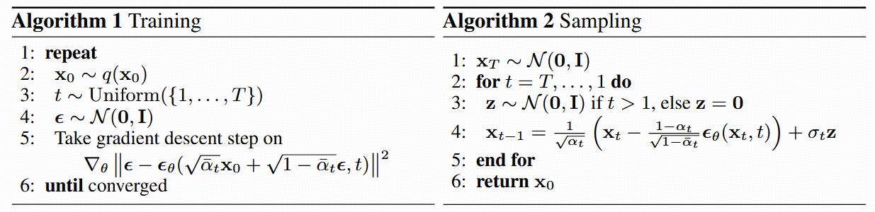
$${\tilde{\mu }}_{t-1}=\frac{1}{\sqrt{a_t}}\left(x_t-\frac{{\beta }_t}{\sqrt{1-{\overline{a}}_t}}{z}_t\right)$$

$z_t$是t时刻的噪声，在推理阶段是未知的，没有公式可以直接求出来，这时候第一步加噪声的步骤开始发力，每一步加的噪声 $z_t$ 是已知的（作为标签），加完噪声的图像 $x_t$ (作为输入)也是已知的，所以作者设计了一个Unet网络模型来预测 $z_t$，得到 $z_t$ 的近似值（神经网络求解其实就是一个最优化过程，用来求解近似值再合适不过），计算loss:
$${\nabla }_{\theta }{\Vert ϵ-{ϵ}_{\theta }\left(\sqrt{{\bar{\alpha }}_t}{x}_0+\sqrt{1-{\bar{\alpha }}_t}ϵ,t\right)\Vert }^2$$
到这一步有了均值和方差就可以得到$x_{t-1}$的分布了，但是要得到论文里的：
$${\mathbf{x}}_{t-1}=\frac{1}{\sqrt{{\alpha }_t}}\left({\mathbf{x}}_t-\frac{1-{\alpha }_t}{\sqrt{1-{\bar{\alpha }}_t}}{\mathbf{ϵ}}_{\theta }({\mathbf{x}}_t,t)\right)+{\sigma }_t\mathbf{z}$$

还有一个优化过程，这一段公式推理龙老师没讲，我自己找了一篇博客看了一下，感觉有点难懂，需要一些数学功底，有兴趣可以参考扩散模型之DDPM的优化目标部分。

三. 代码实现：

只展示最核心的模块实现，完整代码请访问原作者github仓库或者私信本人

导入依赖包：

import math
from inspect import isfunction
from functools import partial
%matplotlib inline
import matplotlib.pyplot as plt
from tqdm.auto import tqdm
from einops import rearrange
import torch
from torch import nn, einsum
import torch.nn.functional as F

时间步（t）编码：

class SinusoidalPositionEmbeddings(nn.Module):def __init__(self, dim):super().__init__()self.dim = dimdef forward(self, time):device = time.devicehalf_dim = self.dim // 2embeddings = math.log(10000) / (half_dim - 1)embeddings = torch.exp(torch.arange(half_dim, device=device) * -embeddings)embeddings = time[:, None] * embeddings[None, :]embeddings = torch.cat((embeddings.sin(), embeddings.cos()), dim=-1)return embeddings# 实例化模块
embed_fn = SinusoidalPositionEmbeddings(dim=8)# 输入时间步 t，形状为 (batch_size,)
t = torch.tensor([1.0, 10.0, 100.0])  # 3个样本# 输出嵌入
output = embed_fn(t)print("Output shape:", output.shape)       # [3, 8]
print("Output:\n", output)

Unet网络，具体实现引用了 ConvNext网络结构

class Unet(nn.Module):def __init__(self,dim,init_dim=None,out_dim=None,dim_mults=(1, 2, 4, 8),channels=3,with_time_emb=True,resnet_block_groups=8,use_convnext=True,convnext_mult=2,):super().__init__()# determine dimensionsself.channels = channelsinit_dim = default(init_dim, dim // 3 * 2)self.init_conv = nn.Conv2d(channels, init_dim, 7, padding=3)dims = [init_dim, *map(lambda m: dim * m, dim_mults)]in_out = list(zip(dims[:-1], dims[1:]))ConvNextif use_convnext:block_klass = partial(ConvNextBlock, mult=convnext_mult)else:block_klass = partial(ResnetBlock, groups=resnet_block_groups)# time embeddingsif with_time_emb:time_dim = dim * 4self.time_mlp = nn.Sequential(SinusoidalPositionEmbeddings(dim),nn.Linear(dim, time_dim),nn.GELU(),nn.Linear(time_dim, time_dim),)else:time_dim = Noneself.time_mlp = None# layersself.downs = nn.ModuleList([])self.ups = nn.ModuleList([])num_resolutions = len(in_out)for ind, (dim_in, dim_out) in enumerate(in_out):is_last = ind >= (num_resolutions - 1)self.downs.append(nn.ModuleList([block_klass(dim_in, dim_out, time_emb_dim=time_dim),block_klass(dim_out, dim_out, time_emb_dim=time_dim),Residual(PreNorm(dim_out, LinearAttention(dim_out))),Downsample(dim_out) if not is_last else nn.Identity(),]))mid_dim = dims[-1]self.mid_block1 = block_klass(mid_dim, mid_dim, time_emb_dim=time_dim)self.mid_attn = Residual(PreNorm(mid_dim, Attention(mid_dim)))self.mid_block2 = block_klass(mid_dim, mid_dim, time_emb_dim=time_dim)for ind, (dim_in, dim_out) in enumerate(reversed(in_out[1:])):is_last = ind >= (num_resolutions - 1)self.ups.append(nn.ModuleList([block_klass(dim_out * 2, dim_in, time_emb_dim=time_dim),block_klass(dim_in, dim_in, time_emb_dim=time_dim),Residual(PreNorm(dim_in, LinearAttention(dim_in))),Upsample(dim_in) if not is_last else nn.Identity(),]))out_dim = default(out_dim, channels)self.final_conv = nn.Sequential(block_klass(dim, dim), nn.Conv2d(dim, out_dim, 1))def forward(self, x, time):x = self.init_conv(x)t = self.time_mlp(time) if exists(self.time_mlp) else Noneh = []# downsamplefor block1, block2, attn, downsample in self.downs:x = block1(x, t)x = block2(x, t)x = attn(x)h.append(x)x = downsample(x)# bottleneckx = self.mid_block1(x, t)x = self.mid_attn(x)x = self.mid_block2(x, t)# upsamplefor block1, block2, attn, upsample in self.ups:x = torch.cat((x, h.pop()), dim=1)x = block1(x, t)x = block2(x, t)x = attn(x)x = upsample(x)return self.final_conv(x)

计算 ${\alpha }_t$和 ${\beta }_t$以及公式中的已知量：

timesteps = 200# define beta schedule
betas = linear_beta_schedule(timesteps=timesteps)# define alphas 
alphas = 1. - betas
alphas_cumprod = torch.cumprod(alphas, axis=0)
alphas_cumprod_prev = F.pad(alphas_cumprod[:-1], (1, 0), value=1.0)
sqrt_recip_alphas = torch.sqrt(1.0 / alphas)# calculations for diffusion q(x_t | x_{t-1}) and others
sqrt_alphas_cumprod = torch.sqrt(alphas_cumprod)
sqrt_one_minus_alphas_cumprod = torch.sqrt(1. - alphas_cumprod)# calculations for posterior q(x_{t-1} | x_t, x_0)
posterior_variance = betas * (1. - alphas_cumprod_prev) / (1. - alphas_cumprod)def extract(a, t, x_shape):batch_size = t.shape[0]out = a.gather(-1, t.cpu())return out.reshape(batch_size, *((1,) * (len(x_shape) - 1))).to(t.device)

图像加噪过程：

def q_sample(x_start, t, noise=None):if noise is None:noise = torch.randn_like(x_start)sqrt_alphas_cumprod_t = extract(sqrt_alphas_cumprod, t, x_start.shape)sqrt_one_minus_alphas_cumprod_t = extract(sqrt_one_minus_alphas_cumprod, t, x_start.shape)return sqrt_alphas_cumprod_t * x_start + sqrt_one_minus_alphas_cumprod_t * noise

计算损失：

def p_losses(denoise_model, x_start, t, noise=None, loss_type="l1"):if noise is None:noise = torch.randn_like(x_start)x_noisy = q_sample(x_start=x_start, t=t, noise=noise)predicted_noise = denoise_model(x_noisy, t)if loss_type == 'l1':loss = F.l1_loss(noise, predicted_noise)elif loss_type == 'l2':loss = F.mse_loss(noise, predicted_noise)elif loss_type == "huber":loss = F.smooth_l1_loss(noise, predicted_noise)else:raise NotImplementedError()return loss

训练Unet

from torchvision.utils import save_imageepochs = 5for epoch in range(epochs):for step, batch in enumerate(dataloader):optimizer.zero_grad()batch_size = batch["pixel_values"].shape[0]batch = batch["pixel_values"].to(device)# Algorithm 1 line 3: sample t uniformally for every example in the batcht = torch.randint(0, timesteps, (batch_size,), device=device).long()loss = p_losses(model, batch, t, loss_type="huber")if step % 100 == 0:print("Loss:", loss.item())loss.backward()optimizer.step()# save generated imagesif step != 0 and step % save_and_sample_every == 0:milestone = step // save_and_sample_everybatches = num_to_groups(4, batch_size)all_images_list = list(map(lambda n: sample(model, batch_size=n, channels=channels), batches))all_images = torch.cat(all_images_list, dim=0)all_images = (all_images + 1) * 0.5save_image(all_images, str(results_folder / f'sample-{milestone}.png'), nrow = 6)

去噪推理过程：

@torch.no_grad()
def p_sample(model, x, t, t_index):betas_t = extract(betas, t, x.shape)sqrt_one_minus_alphas_cumprod_t = extract(sqrt_one_minus_alphas_cumprod, t, x.shape)sqrt_recip_alphas_t = extract(sqrt_recip_alphas, t, x.shape)# Equation 11 in the paper# Use our model (noise predictor) to predict the meanmodel_mean = sqrt_recip_alphas_t * (x - betas_t * model(x, t) / sqrt_one_minus_alphas_cumprod_t)if t_index == 0:return model_meanelse:posterior_variance_t = extract(posterior_variance, t, x.shape)noise = torch.randn_like(x)# Algorithm 2 line 4:return model_mean + torch.sqrt(posterior_variance_t) * noise # Algorithm 2 but save all images:
@torch.no_grad()
def p_sample_loop(model, shape):device = next(model.parameters()).deviceb = shape[0]# start from pure noise (for each example in the batch)img = torch.randn(shape, device=device)imgs = []for i in tqdm(reversed(range(0, timesteps)), desc='sampling loop time step', total=timesteps):img = p_sample(model, img, torch.full((b,), i, device=device, dtype=torch.long), i)imgs.append(img.cpu().numpy())return imgs@torch.no_grad()
def sample(model, image_size, batch_size=16, channels=3):return p_sample_loop(model, shape=(batch_size, channels, image_size, image_size))samples = sample(model, image_size=image_size, batch_size=64, channels=channels)