Python打卡训练营Day37
DAY 37 早停策略和模型权重的保存
知识点回顾:
- 过拟合的判断:测试集和训练集同步打印指标
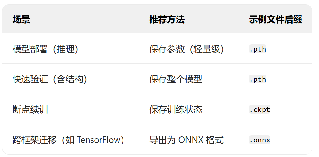
- 模型的保存和加载
- 仅保存权重
- 保存权重和模型
- 保存全部信息checkpoint,还包含训练状态
- 早停策略

作业:对信贷数据集训练后保存权重,加载权重后继续训练50轮,并采取早停策略
#数据预处理
import pandas as pd
import seaborn as sns
import matplotlib.pyplot as plt
plt.rcParams['font.sans-serif'] = ['SimHei']
plt.rcParams['axes.unicode_minus'] = False
dt = pd.read_csv(r'data.csv')
dt.head()
dt.info()
dt.isnull().sum()#缺失值处理
discrete_features = []
continuous_features = []
for feature in dt.columns:if dt[feature].dtype == 'object':discrete_features.append(feature)else:continuous_features.append(feature)
print(f'离散特征:{discrete_features}')
print(f'连续特征:{continuous_features}')for features in discrete_features:mode_value = dt[features].mode()[0]dt[features].fillna(mode_value,inplace=True)print(f"列 '{features}' 使用众数 {mode_value} 填补空值")for features in continuous_features:median_value = dt[features].median()dt[features].fillna(median_value,inplace=True)print(f"列 '{features}' 使用中位数 {median_value} 填补空值")#离散特征做标签编码/独热编码
dt["Home Ownership"].value_counts()
dt['Years in current job'].value_counts()
dt['Purpose'].value_counts()
dt['Term'].value_counts()
mapping = {'Home Ownership': {'Own Home': 0,'Rent': 1,'Have Mortgage': 2,'Home Mortgage': 3},'Term': {'Short Term': 0,'Long Term': 1},'Purpose': {'debt_consolidation': 2,'buy house': 1,'business loan': 1,'major purchase': 1,'small business': 1,'other': 0,'home improvements': 0,'buy a car': 0,'medical bills': 0,'take a trip': 0,'wedding': 0,'moving': 0,'educational expenses': 0,'vacation': 0,'renewable energy': 0},'Years in current job': {'10+ years': 0,'9 years': 1,'8 years': 1,'7 years': 2,'6 years': 2,'5 years': 3,'4 years': 3,'3 years': 4,'2 years': 4,'< 1 year': 5}
}dt["Home Ownership"] = dt["Home Ownership"].map(mapping["Home Ownership"])
dt["Term"] = dt["Term"].map(mapping["Term"])
dt["Purpose"] = dt["Purpose"].map(mapping["Purpose"])
dt["Years in current job"] = dt["Years in current job"].map(mapping["Years in current job"])
dt.head()
dt = dt.drop(['Purpose','Id'],axis=1)import torch
import torch.nn as nn
import torch.optim as optim
from sklearn.datasets import load_iris
from sklearn.model_selection import train_test_split
from sklearn.preprocessing import MinMaxScaler
import time
import matplotlib.pyplot as pltX = dt.drop('Credit Default', axis=1)  # 特征
y = dt['Credit Default']  # 标签# 划分训练集和测试集
X_train, X_test, y_train, y_test = train_test_split(X, y, test_size=0.2, random_state=42)
# 归一化数据
scaler = MinMaxScaler()
X_train = scaler.fit_transform(X_train)
X_test = scaler.transform(X_test)# 将数据转换为PyTorch张量
X_train = torch.FloatTensor(X_train)
y_train = torch.LongTensor(y_train.to_numpy())
X_test = torch.FloatTensor(X_test)
y_test = torch.LongTensor(y_test.to_numpy())# 检查数据合法性
assert torch.isnan(X_train).sum() == 0, "X_train 包含 NaN"
assert torch.unique(y_train).tolist() == [0, 1], "标签应为 0 或 1"
#特征有多少列
print(X_train.shape[1])# 定义神经网络模型
class MLP(nn.Module):def __init__(self):super(MLP, self).__init__()self.fc1 = nn.Linear(15, 30)  # 输入层到隐藏层 15个特征,30个神经元self.relu = nn.ReLU()self.dropout = nn.Dropout(0.3)  # 添加Dropout防止过拟合self.fc2 = nn.Linear(30, 2)  # 隐藏层到输出层 30个神经元,2个类别def forward(self, x):out = self.fc1(x)out = self.relu(out)out = self.dropout(out)  # 应用Dropoutout = self.fc2(out)return out
# 实例化模型、损失函数和优化器
model = MLP()
criterion = nn.CrossEntropyLoss()  # 多分类问题,使用交叉熵损失函数
optimizer = optim.Adam(model.parameters(), lr=0.0001)  # 使用Adam优化器
# 训练模型
num_epochs = 20000  # 训练的轮数# 用于存储每200个epoch的损失值和对应的epoch数
train_losses = [] # 存储训练集损失
test_losses = [] # 新增:存储测试集损失
epochs = []from tqdm import tqdm  # 导入tqdm库用于进度条显示start_time = time.time()  # 记录开始时间# 创建tqdm进度条
with tqdm(total=num_epochs, desc="训练进度", unit="epoch") as pbar:# 训练模型for epoch in range(num_epochs):# 前向传播outputs = model(X_train)  # 隐式调用forward函数train_loss = criterion(outputs, y_train)# 反向传播和优化optimizer.zero_grad()train_loss.backward()optimizer.step()# 记录损失值并更新进度条if (epoch + 1) % 200 == 0:#计算测试集损失,新增代码model.eval()with torch.no_grad():test_outputs = model(X_test)test_loss = criterion(test_outputs, y_test)model.train()train_losses.append(train_loss.item())test_losses.append(test_loss.item())epochs.append(epoch + 1)# 更新进度条的描述信息pbar.set_postfix({'Train Loss': f'{train_loss.item():.4f}', 'Test Loss': f'{test_loss.item():.4f}'})# 每1000个epoch更新一次进度条if (epoch + 1) % 1000 == 0:pbar.update(1000)  # 更新进度条# 确保进度条达到100%if pbar.n < num_epochs:pbar.update(num_epochs - pbar.n)  # 计算剩余的进度并更新
time_all = time.time() - start_time  # 计算训练时间
print(f'Training time: {time_all:.2f} seconds')
# 可视化损失曲线
plt.figure(figsize=(10, 6))
plt.plot(epochs, train_losses, label='Train Loss') # 原始代码已有
plt.plot(epochs, test_losses, label='Test Loss')  # 新增:测试集损失曲线
plt.xlabel('Epoch')
plt.ylabel('Loss')
plt.title('Training and Test Loss over Epochs')
plt.legend() # 新增:显示图例
plt.grid(True)
plt.show()# 测试模型
model.eval()  # 设置模型为评估模式,不进行梯度计算
with torch.no_grad():  # 不计算梯度,减少内存消耗outputs = model(X_test)  # 对测试集进行预测_, predicted = torch.max(outputs, 1)  # 找到概率最大的类别correct = (predicted == y_test).sum().item()  # 计算正确预测的数量total = y_test.size(0)  # 测试集样本总数accuracy = correct / total  # 计算准确率print(f'Test Accuracy: {accuracy*100:.2f}%')# 模型的保存和加载
# 1.仅保存模型参数(推荐)
torch.save(model.state_dict(), 'credit_default_model.pth')  # 保存模型参数
# 加载模型
model = MLP()  # 创建模型实例
model.load_state_dict(torch.load('credit_default_model.pth'))  # 加载模型参数
# model.eval()  # 切换至推理模式(可选)
# 2.保存模型+权重
torch.save(model, 'credit_default_model_full.pth')  # 保存整个模型,包括结构和参数
# 加载模型
model = torch.load('credit_default_model_full.pth')  # 加载整个模型
# model.eval()  # 切换至推理模式(可选)
# 3.保存训练状态(断点续训)
# checkpoint = {
#     "model_state_dict": model.state_dict(),
#     "optimizer_state_dict": optimizer.state_dict(),
#     "epoch": epoch,
#     "loss": best_loss,
# }
# torch.save(checkpoint, "checkpoint.pth")# # 加载并续训
# model = MLP()
# optimizer = torch.optim.Adam(model.parameters())
# checkpoint = torch.load("checkpoint.pth")# model.load_state_dict(checkpoint["model_state_dict"])
# optimizer.load_state_dict(checkpoint["optimizer_state_dict"])
# start_epoch = checkpoint["epoch"] + 1  # 从下一轮开始训练
# best_loss = checkpoint["loss"]# # 继续训练循环
# for epoch in range(start_epoch, num_epochs):
#     train(model, optimizer, ...)#work:保存上述训练的权重并加载权重后继续训练50轮,启用早停策略
#torch.save(model, 'credit_default_model_full.pth')  # 保存整个模型,包括结构和参数
# 加载模型
model = torch.load('credit_default_model_full.pth')  # 加载整个模型
# 分类问题使用交叉熵损失函数
criterion = nn.CrossEntropyLoss()optimizer = optim.Adam(model.parameters(), lr=0.0001)  # 使用Adam优化器# 训练模型
num_epochs = 50  # 训练的轮数# 用于存储每5个epoch的损失值和对应的epoch数
train_losses = []  # 存储训练集损失
test_losses = []   # 存储测试集损失
epochs = []# ===== 新增早停相关参数 =====
best_test_loss = float('inf')  # 记录最佳测试集损失
best_epoch = 0                 # 记录最佳epoch
patience = 5                # 早停耐心值(连续多少轮测试集损失未改善时停止训练)
counter = 0                    # 早停计数器
early_stopped = False          # 是否早停标志
# ==========================start_time = time.time()  # 记录开始时间# 创建tqdm进度条
with tqdm(total=num_epochs, desc="训练进度", unit="epoch") as pbar:# 训练模型for epoch in range(num_epochs):# 前向传播outputs = model(X_train)  # 隐式调用forward函数train_loss = criterion(outputs, y_train)# 反向传播和优化optimizer.zero_grad()train_loss.backward()optimizer.step()# 记录损失值并更新进度条if (epoch + 1) % 10 == 0:# 计算测试集损失model.eval()with torch.no_grad():test_outputs = model(X_test)test_loss = criterion(test_outputs, y_test)model.train()train_losses.append(train_loss.item())test_losses.append(test_loss.item())epochs.append(epoch + 1)# 更新进度条的描述信息pbar.set_postfix({'Train Loss': f'{train_loss.item():.4f}', 'Test Loss': f'{test_loss.item():.4f}'})# ===== 新增早停逻辑 =====if test_loss.item() < best_test_loss: # 如果当前测试集损失小于最佳损失best_test_loss = test_loss.item() # 更新最佳损失best_epoch = epoch + 1 # 更新最佳epochcounter = 0 # 重置计数器# 保存最佳模型torch.save(model.state_dict(), 'best_credit_default_model.pth')else:counter += 1if counter >= patience:print(f"早停触发!在第{epoch+1}轮,测试集损失已有{patience}轮未改善。")print(f"最佳测试集损失出现在第{best_epoch}轮,损失值为{best_test_loss:.4f}")early_stopped = Truebreak  # 终止训练循环# ======================# 每10个epoch更新一次进度条if (epoch + 1) % 10 == 0:pbar.update(10)  # 更新进度条# 确保进度条达到100%if pbar.n < num_epochs:pbar.update(num_epochs - pbar.n)  # 计算剩余的进度并更新time_all = time.time() - start_time  # 计算训练时间
print(f'Training time: {time_all:.2f} seconds')# ===== 新增:加载最佳模型用于最终评估 =====
if early_stopped:print(f"加载第{best_epoch}轮的最佳模型进行最终评估...")model.load_state_dict(torch.load('best_credit_default_model.pth'))
# ================================# 可视化损失曲线
plt.figure(figsize=(10, 6))
plt.plot(epochs, train_losses, label='Train Loss')
plt.plot(epochs, test_losses, label='Test Loss')
plt.xlabel('Epoch')
plt.ylabel('Loss')
plt.title('Training and Test Loss over Epochs')
plt.legend()
plt.grid(True)
plt.show()# 在测试集上评估模型
model.eval()
with torch.no_grad():outputs = model(X_test)_, predicted = torch.max(outputs, 1)correct = (predicted == y_test).sum().item()accuracy = correct / y_test.size(0)print(f'测试集准确率: {accuracy * 100:.2f}%') 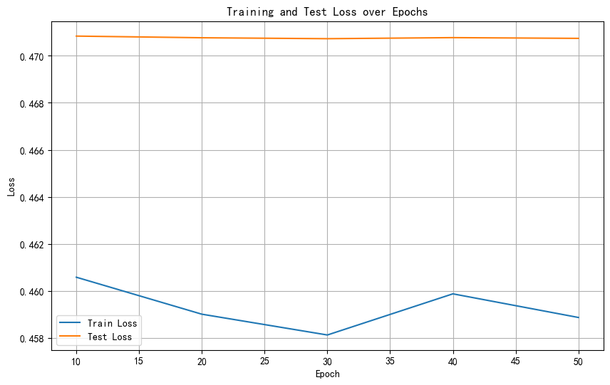
训练数据在波动表示其可能陷入局部最优解中不稳定,而测试数据趋于稳定表示已近乎拟合或模型性能已到极限。
@浙大疏锦行-CSDN博客