基于Seurat的空转单样本数据分析流程学习(一)
本次分析使用的数据集是:GSE281978,选择了其中的一个数据GSM8633891进行分析;
分析流程
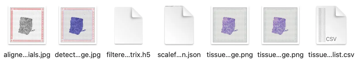
aligned_fiducials.jpg:带有芯片定位点(fiducial markers)的图像。这些定位点是Visium芯片上的参照标记,用来帮助显微镜图像与芯片的spot array对齐;在图像配准过程中保证组织切片位置与空间条码坐标准确匹配。
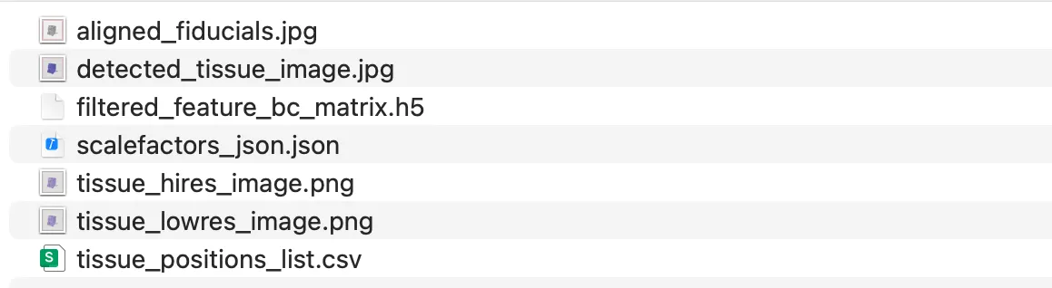
detected_tissue_image.jpg:组织识别后的二值图像。用于标记哪些区域包含组织(组织蒙版 mask),帮助区分组织区域和背景区域;常用于筛选有效的 spots。
filtered_feature_bc_matrix.h5:核心的基因表达矩阵文件(HDF5 格式)。行表示基因,列表示空间位置(spot/barcode),数值为UMI counts;该矩阵已去除低质量基因和低质量spot,是Seurat、Scanpy等空间分析的主要输入。
scalefactors_json.json:存放图像与空间坐标之间的缩放因子。主要字段包括高/低分辨率图像的缩放比例和spot 在原始图像上的直径;用于将spot坐标准确映射到组织切片图像上,保证可视化时位置匹配。
tissue_hires_image.png:高分辨率 H&E 染色组织切片图像。用于在空间可视化中叠加基因表达信息,生成高质量的展示图像。
tissue_lowres_image.png:低分辨率 H&E 染色组织切片图像。常用于快速加载和浏览,在交互式分析中默认使用,节省内存和计算资源。
tissue_positions_list.csv:每个 spot 的空间位置信息文件。包括 spot 的条码、是否位于组织区域(1=组织内,0=背景)、芯片阵列上的行列位置以及在图像中的像素坐标;用于确定每个 spot 在组织图像上的具体位置。
在空间转录组分析中,必要的文件包括 filtered_feature_bc_matrix.h5(基因表达矩阵)、tissue_positions_list.csv(spot的空间位置信息)、scalefactors_json.json(坐标与图像的缩放比例)以及 tissue_lowres_image.png 或 tissue_hires_image.png(组织切片图像,用于可视化)。
1.导入
rm(list = ls())
library(Seurat)
library(future)
library(ggplot2)
library(hdf5r)setwd("0-GSM8633891")
把GSM8633891数据集整理成了这样的一个文件结构,并且把名称进行修改。由于空转数据基本上都是一个个处理,所以手动解压、改名、移动可能更快。
2.单样本读取数据
data <- Read10X_h5("./GSM8633891/filtered_feature_bc_matrix.h5")
dim(data)
# [1] 36601  1187object <- CreateSeuratObject(counts = data, assay = "Spatial", min.cells = 3, #过滤在少于3个细胞中表达的基因,以减少低表达基因的干扰project = "GSM8633891")
object
#An object of class Seurat
#20050 features across 1187 samples within 1 assay
#Active assay: Spatial (20050 features, 0 variable features)
# 1 layer present: counts# 再读取
image <- Read10X_Image(image.dir = "GSM8633891/", image.name = "tissue_hires_image.png",filter.matrix = TRUE)
image
#Spatial coordinates for 1187 cells
#Default segmentation boundary: centroids
#Associated assay: Spatial
#Key: slice1_
dim(image)image <- image[Cells(x = object)]
DefaultAssay(object = image) <- "Spatial"# 添加图片到object中
object[["GSM8633891"]] <- image
# 通常分析采用高分辨率图像,为了后续不报错,把缩放因子都统一一下
object@images[["GSM8633891"]]@scale.factors$lowres <- object@images[["GSM8633891"]]@scale.factors$hiressce.all <- object
## 简单探索一下数据结构
as.data.frame(sce.all[["Spatial"]]$counts[1:4,1:4])
#           AAACCGTTCGTCCAGG-1 AAACGAGACGGTTGAT-1 AAACTGCTGGCTCCAA-1 AAAGGCTACGGACCAT-1
#AL627309.1                  0                  0                  0                  0
#LINC01409                   0                  0                  0                  0
#LINC01128                   0                  1                  2                  0
#LINC00115                   0                  0                  0                  0
as.data.frame(LayerData(sce.all, assay = "Spatial", layer = "counts")[1:5,1:5])
#           AAACCGTTCGTCCAGG-1 AAACGAGACGGTTGAT-1 AAACTGCTGGCTCCAA-1 AAAGGCTACGGACCAT-1
#AL627309.1                  0                  0                  0                  0
#LINC01409                   0                  0                  0                  0
#LINC01128                   0                  1                  2                  0
#LINC00115                   0                  0                  0                  0
#FAM41C                      0                  0                  0                  0
#           AAAGGCTCTCGCGCCG-1
#AL627309.1                  0
#LINC01409                   0
#LINC01128                   0
#LINC00115                   0
#FAM41C                      0
head(sce.all@meta.data)
#                   orig.ident nCount_Spatial nFeature_Spatial
#AAACCGTTCGTCCAGG-1 GSM8633891          13545             3293
#AAACGAGACGGTTGAT-1 GSM8633891          34745             7358
#AAACTGCTGGCTCCAA-1 GSM8633891          19470             5548
#AAAGGCTACGGACCAT-1 GSM8633891          20883             5933
#AAAGGCTCTCGCGCCG-1 GSM8633891          18630             5219
#AAAGGGATGTAGCAAG-1 GSM8633891          27316             6667
table(sce.all$orig.ident)
#GSM8633891
#      1187
Layers(sce.all)
# [1] "counts"
Assays(sce.all)
# [1] "Spatial"library(qs)
qsave(sce.all, file="GSM8633891/sce.all.qs")
3.数据预处理
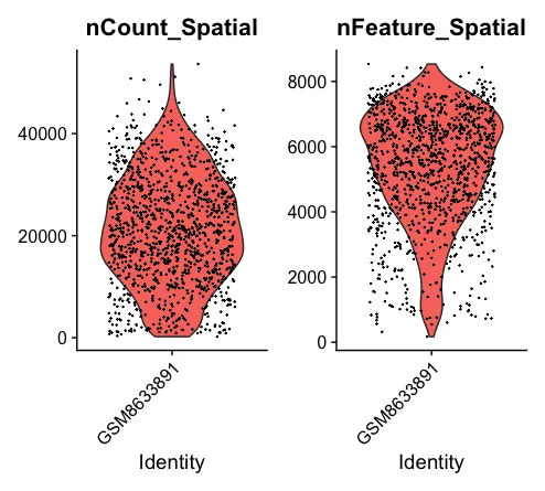
plot1 <- VlnPlot(sce.all, features = c("nCount_Spatial","nFeature_Spatial"), pt.size = 0.1) + NoLegend()
plot1
ggsave(filename = "1-QC/VlnPlot.pdf", width = 12,height = 6, plot = plot1)######
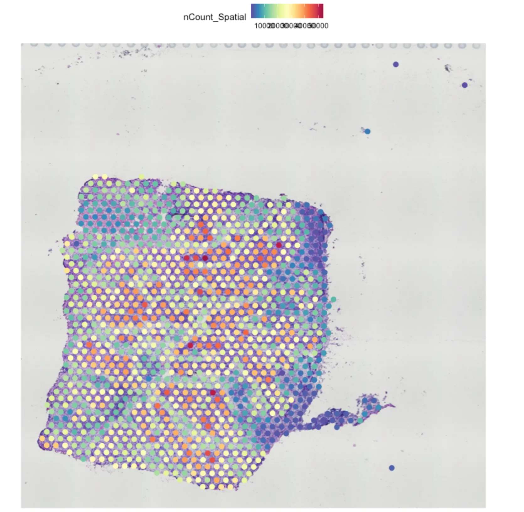
plot2 <- SpatialFeaturePlot(sce.all, features = "nCount_Spatial",pt.size.factor = 2)
plot2
ggsave(filename = "1-QC/FeaturePlot_nCount.pdf", width = 18,height = 6, plot = plot2)########
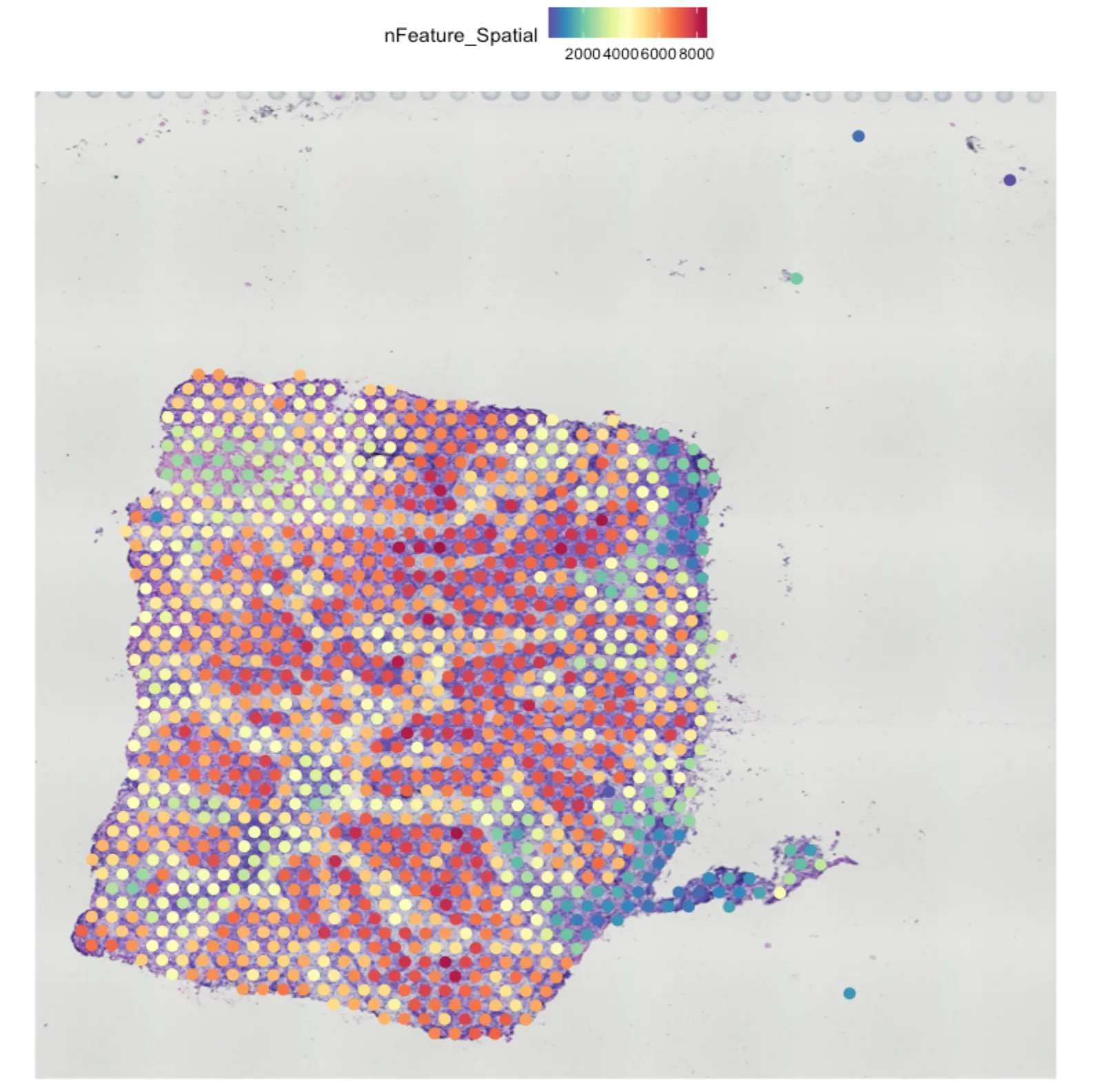
plot3 <- SpatialFeaturePlot(sce.all, features ="nFeature_Spatial",pt.size.factor = 2)
plot3
ggsave(filename ="1-QC/FeaturePlot_nFeature.pdf", width = 18,height = 6, plot = plot3)
5.过滤SPOT
## 过滤spot
sce.all <- subset(sce.all, subset = nFeature_Spatial > 200 )### 计算线粒体/核糖体/特定基因集的比例
#mito_genes <- grep("^MT-", rownames(sce.all),ignore.case = T, value = T)
## 可能是13个线粒体基因
#print(mito_genes)
#sce.all <- PercentageFeatureSet(sce.all,
#                                features = mito_genes,
#                                col.name = "percent_mito")
6.标准化
sce.all <- SCTransform(sce.all, assay ="Spatial", verbose = T)
sce.all <- RunPCA(sce.all, assay ="SCT", verbose = FALSE)
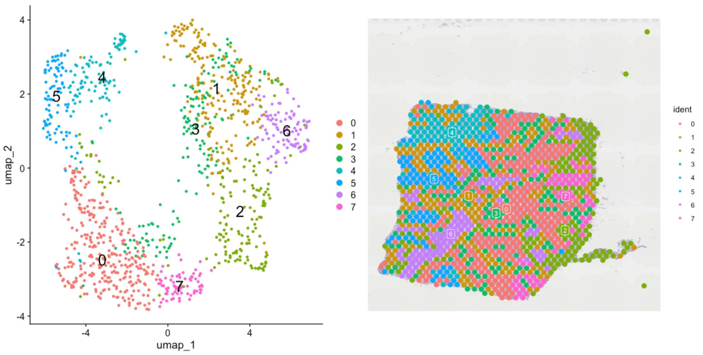
sce.all <- FindNeighbors(sce.all, reduction ="pca", dims = 1:30)
sce.all <- FindClusters(sce.all, verbose = FALSE,resolution = 0.8)
sce.all <- RunUMAP(sce.all, reduction ="pca", dims = 1:30)p1 <- DimPlot(sce.all, reduction ="umap", label = TRUE,label.size = 7);p1
ggsave(filename ="1-QC/DimPlot.pdf", width = 9,height = 6, plot = p1)p2 <- SpatialDimPlot(sce.all, label = TRUE, label.size = 3,pt.size.factor = 2,image.alpha = 0.6);p2
ggsave(filename ="1-QC/SpatialDimPlot.pdf", width = 18,height = 6, plot = p2)p1|p2
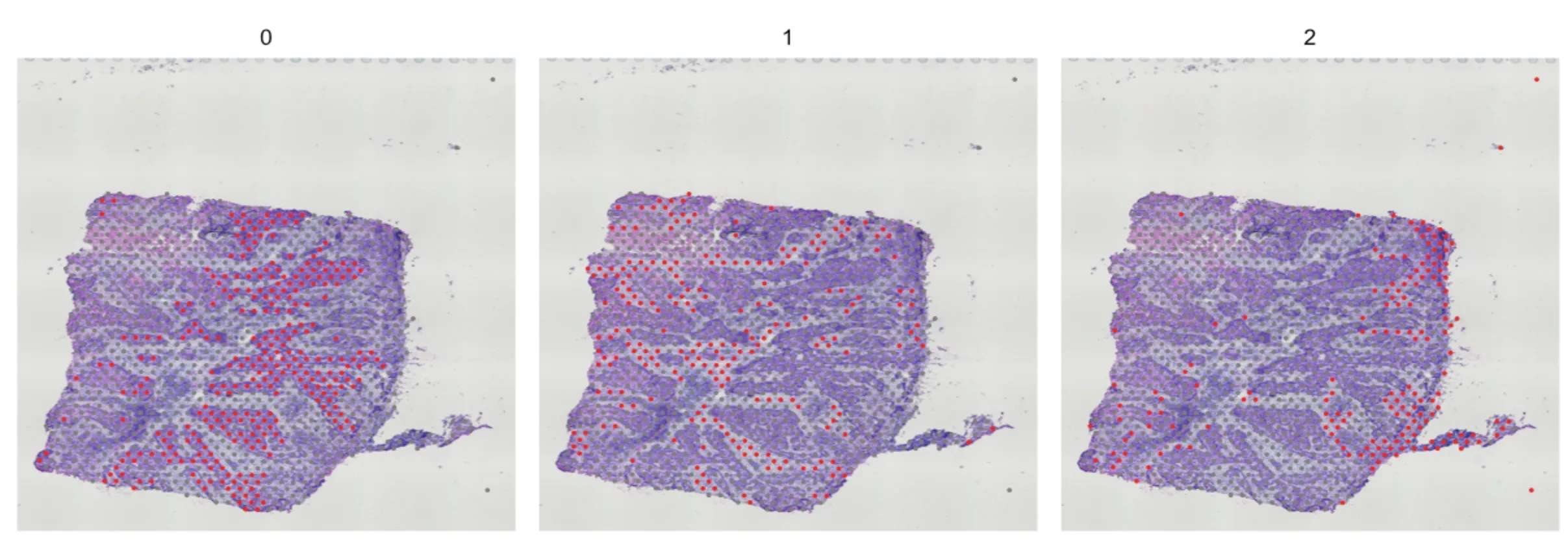
6.0 提取相应的ident组分
SpatialDimPlot(sce.all, cells.highlight = CellsByIdentities(object = sce.all, idents = c(0,1,2)),facet.highlight = TRUE, ncol = 3)SpatialDimPlot(sce.all, label = TRUE, label.size = 3)
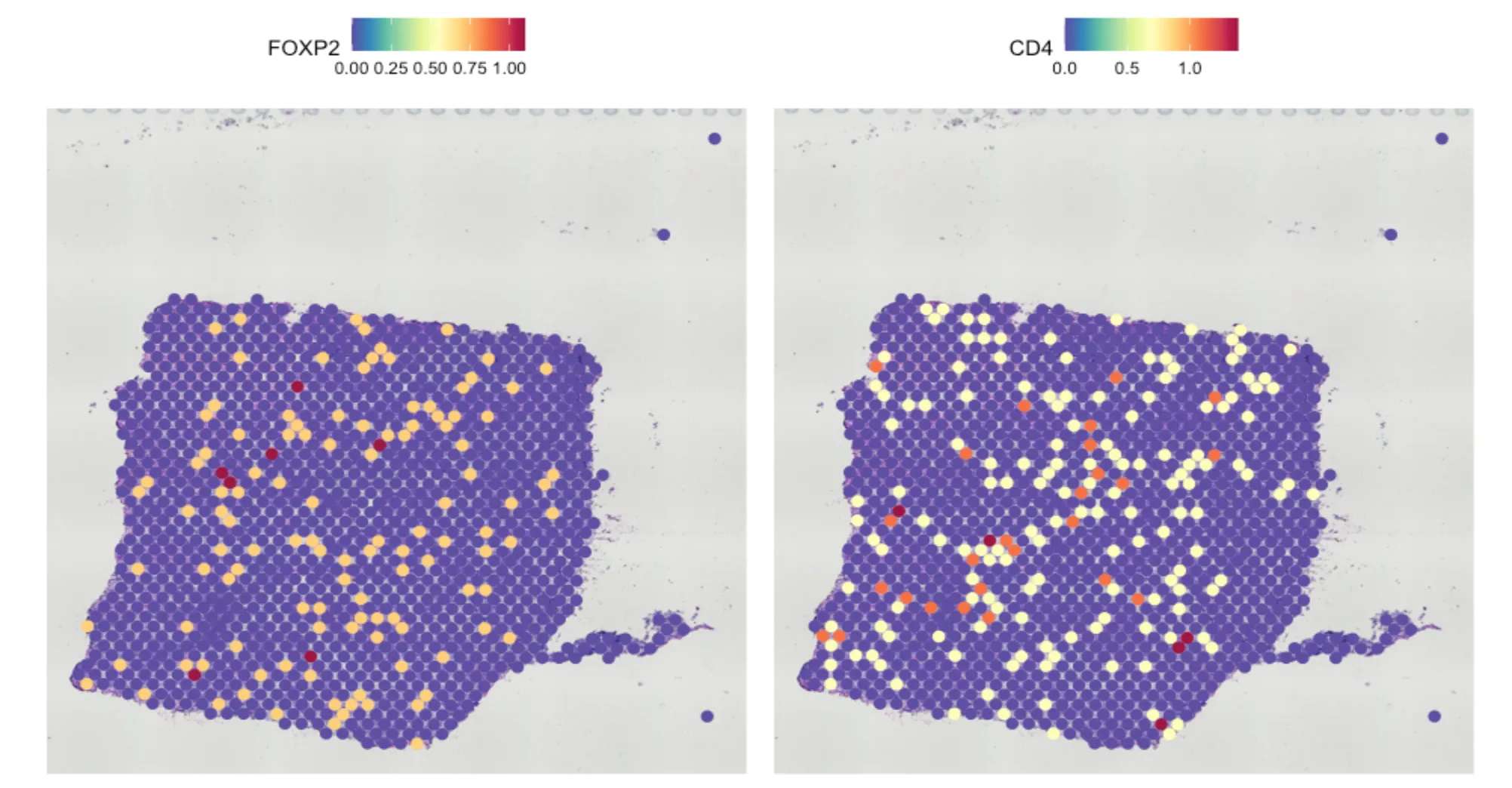
6.1 基因可视化
SpatialFeaturePlot(sce.all, features = c("FOXP2", "CD4"),pt.size = 4)
7.空间变异特征识别
### 第一种方法:选择特定ident进行差异表达分析
de_markers <- FindMarkers(sce.all, ident.1 = 5, ident.2 = 6)
SpatialFeaturePlot(object = sce.all, features = rownames(de_markers)[1:3], alpha = c(0.1, 1), ncol = 2)### 第二种方法:实现无注释情况下探索表现出空间模式性的特征
### 默认方法 method = 'markvariogram
sce.all <- FindSpatiallyVariableFeatures(sce.all,assay = "SCT", features = VariableFeatures(sce.all)[1:1000],selection.method = "moransi")
top.features <- head(SpatiallyVariableFeatures(sce.all, selection.method = "moransi"), 3)
SpatialFeaturePlot(sce.all, features = top.features, ncol = 2, alpha = c(0.1, 1))
8.基于现有单细胞数据集去映射
在Visium实验中,每个spot的直径约为50微米,因此其捕获的转录组信号往往来源于多个细胞。对于那些已有单细胞转录组(scRNA-seq)数据的系统,研究者通常希望对这些空间voxels进行去卷积(deconvolution),以预测其中潜在的细胞类型组成。
采用了在Seurat v3 中引入的“anchor”整合工作流程,能够实现从参考数据集向查询数据集的概率性注释转移。具体而言,在这里使用标签转移(label transfer)流程,并结合 sctransform 标准化方法。
# 读取参考数据集(整理好的头颈癌示例数据集)
library(qs)
ref <- qread(".././0-reference/sce_celltype.qs")
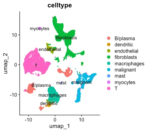
# 该注释存储在meta数据的“celltype”列中。
DimPlot(ref, group.by = "celltype", label = TRUE)
# 设置ncells=3000 会对整个数据集进行归一化
# 显著提高了 SCTransform 的速度,且不会造成性能损失
library(dplyr)
ref <- SCTransform(ref, ncells = 3000, verbose = FALSE) %>%RunPCA(verbose = FALSE) %>%RunUMAP(dims = 1:30)
# 经过筛选后对空间数据进行重新归一化处理。
sce.all <- SCTransform(sce.all, assay = "Spatial", verbose = FALSE) %>%RunPCA(verbose = FALSE)# 找到anchors
anchors <- FindTransferAnchors(reference = ref, query = sce.all, # 指定被预测细胞类型的数据normalization.method = "SCT")
#Normalizing query using reference SCT model
#Warning: No layers found matching search pattern provided
#Only one SCT model detected; no need to select.
#Performing PCA on the provided reference using 2739 features as input.
#Projecting cell embeddings
#Finding neighborhoods
#Finding anchors
#Found 641 anchorspredictions.assay <- TransferData(anchorset = anchors, refdata = ref$celltype,prediction.assay = TRUE,weight.reduction = sce.all[["pca"]], dims = 1:30)
sce.all[["predictions"]] <- predictions.assayDefaultAssay(sce.all) <- "predictions"
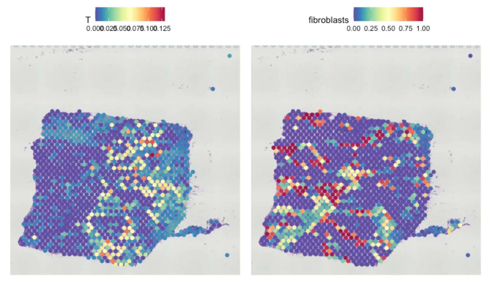
SpatialFeaturePlot(sce.all, features = c("T", "fibroblasts"), pt.size.factor = 3, ncol = 2, crop = TRUE)
# 基于这些预测得分,还可以推断出在空间上具有局限性分布的细胞类型。
# 采用相同的基于标记点过程的方法来定义空间可变特征,但这里使用的“标记”不再是基因表达量,而是细胞类型的预测得分。
sce.all <- FindSpatiallyVariableFeatures(sce.all, assay = "predictions", selection.method = "moransi",features = rownames(sce.all), r.metric = 5, slot = "data")
top.clusters <- head(SpatiallyVariableFeatures(sce.all, selection.method = "moransi"), 4)
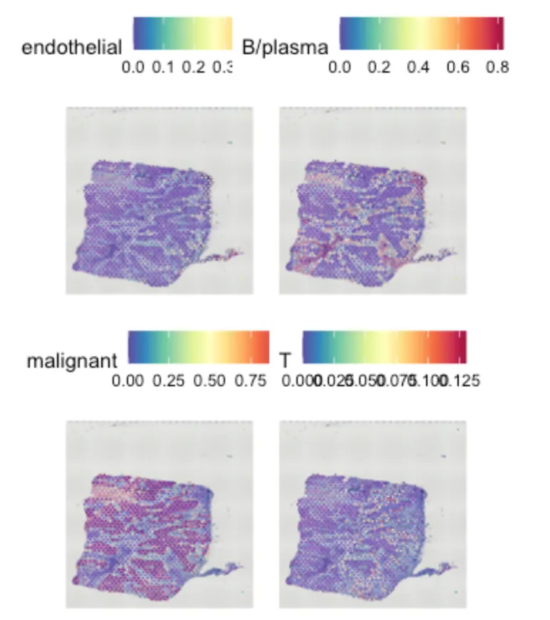
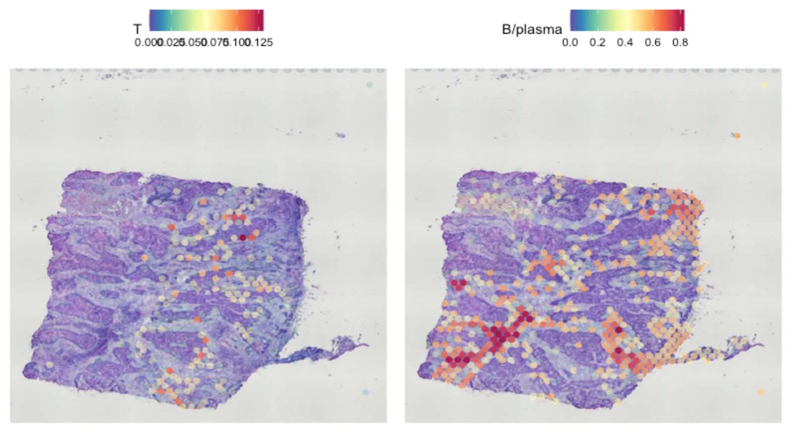
SpatialPlot(object = sce.all, features = top.clusters, ncol = 2)SpatialFeaturePlot(sce.all, features = c("T", "B/plasma"), pt.size.factor = 1, ncol = 2,crop = FALSE, alpha = c(0.1, 1))
排名靠前的cluster
展示特定的cluster
9.使用RCTD(Robust Cell Type Decomposition)进行空间解卷积
library(spacexr)
library(RCTD)# 读取参考数据集
library(qs)
ref <- qread(".././0-reference/sce_celltype.qs")
table(ref$celltype)
# RCTD分析中celltype不能有特殊符号
ref$celltype <- gsub("B/plasma", "B", ref$celltype)ref <- UpdateSeuratObject(ref)
Idents(ref) <- "celltype"# 提取信息以传递给 RCTD Reference 函数
counts <- ref[["RNA"]]$counts
cluster <- as.factor(ref$celltype)
names(cluster) <- colnames(ref)
nUMI <- ref$nCount_RNA
names(nUMI) <- colnames(ref)
reference <- Reference(counts, cluster, nUMI)# 使用SpatialRNA的RCTD函数设置query
counts <- sce.all[["Spatial"]]$counts
coords <- GetTissueCoordinates(sce.all)
colnames(coords) <- c("x", "y")
coords[is.na(colnames(coords))] <- NULL
query <- SpatialRNA(coords, counts, colSums(counts))
9.1 RCTD去卷积
RCTD <- create.RCTD(query, reference, max_cores = 8)
RCTD <- run.RCTD(RCTD, doublet_mode = "doublet")
sce.all <- AddMetaData(sce.all, metadata = RCTD@results$results_df)# 可视化
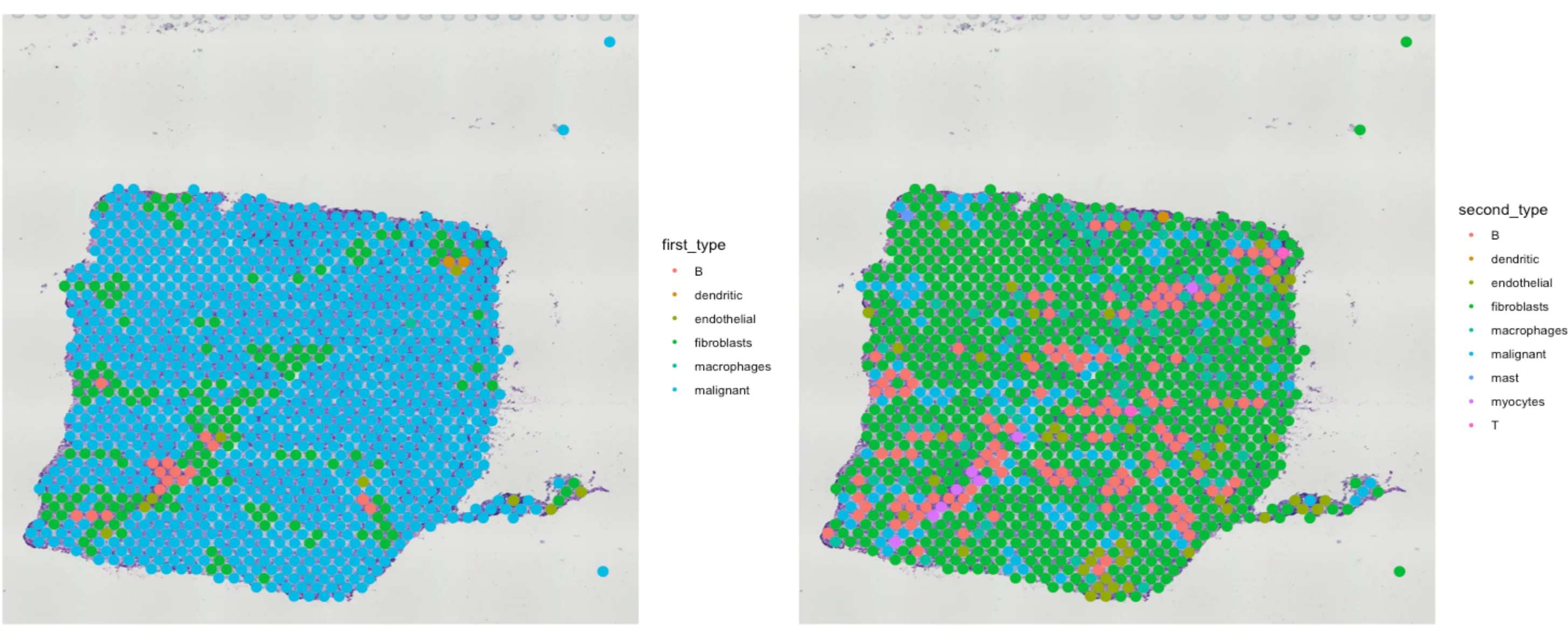
p1 <- SpatialDimPlot(sce.all, group.by = "first_type")
p2 <- SpatialDimPlot(sce.all, group.by = "second_type")
p1 | p2
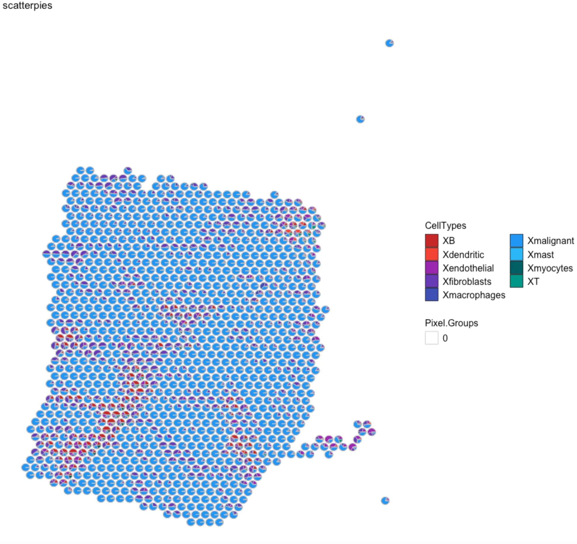
9.2 STdeconvolve可视化
## 借用STdeconvolve绘制一下饼图看看:
library(STdeconvolve)
library(ggplot2)
library(ggsci)
library(spacexr)
library(qs)
RCTD <- qread("RCTD.qs")barcodes <- colnames(RCTD@spatialRNA@counts)
weights <- RCTD@results$weights
norm_weights <- t(apply(weights, 1, function(x) x / sum(x)))
dim(norm_weights)
norm_weights[1:5,1:6]
head(rowSums(as.matrix(norm_weights)))
head(norm_weights)m <- as.matrix(norm_weights)
p <- coords
plt <- vizAllTopics(theta = m,pos = p,topicOrder=seq(ncol(m)),topicCols=rainbow(ncol(m)),groups = NA,group_cols = NA,r = 150, # 散点图的大小;根据像素的坐标进行调整lwd = 0.3,showLegend = TRUE,plotTitle = "scatterpies")## 可以在ggplot2中处理图形
library(paletteer)
my_colors<- c(paletteer_d("awtools::bpalette"),paletteer_d("awtools::a_palette"),paletteer_d("awtools::mpalette"))
plt <- plt + coord_flip() + scale_x_reverse() + ggplot2::guides(fill=ggplot2::guide_legend(ncol=2)) +scale_fill_manual(values = my_colors)
plt
ggsave('Spaital_scatterpies.pdf', width=9, height=7, plot=plt, bg="white")
参考资料
Robust Cell Type Decomposition-RCTD:Robust decomposition of cell type mixtures in spatial transcriptomics. Nat Biotechnol. 2022 Apr;40(4):517-526.
Seuraat-spatital transcriptomic:https://satijalab.org/seurat/articles/spatial_vignette
生信技能树-RCTD可视化:https://mp.weixin.qq.com/s/rwcOTFAZCaIV-i7MGDrOow