当前位置：首页 > news >正文

5.24 打卡

news 2025/5/25 16:03:45

DAY 35 模型可视化与推理

知识点回顾：

三种不同的模型可视化方法：推荐torchinfo打印summary+权重分布可视化
进度条功能：手动和自动写法，让打印结果更加美观
推理的写法：评估模式

作业：调整模型定义时的超参数，对比下效果。

import torch
import torch.nn as nn
import torch.optim as optim
from sklearn.datasets import load_iris
from sklearn.model_selection import train_test_split
from sklearn.preprocessing import MinMaxScaler
import time
import matplotlib.pyplot as plt
from tqdm import tqdm  # 导入tqdm库用于进度条显示# 设置GPU设备
device = torch.device("cuda:0" if torch.cuda.is_available() else "cpu")
print(f"使用设备: {device}")# 加载鸢尾花数据集
iris = load_iris()
X = iris.data  # 特征数据
y = iris.target  # 标签数据# 划分训练集和测试集
X_train, X_test, y_train, y_test = train_test_split(X, y, test_size=0.2, random_state=42)# 归一化数据
scaler = MinMaxScaler()
X_train = scaler.fit_transform(X_train)
X_test = scaler.transform(X_test)# 将数据转换为PyTorch张量并移至GPU
X_train = torch.FloatTensor(X_train).to(device)
y_train = torch.LongTensor(y_train).to(device)
X_test = torch.FloatTensor(X_test).to(device)
y_test = torch.LongTensor(y_test).to(device)# 定义不同结构的MLP模型
class MLP_Baseline(nn.Module):def __init__(self):super(MLP_Baseline, self).__init__()self.fc1 = nn.Linear(4, 10)  # 输入层到隐藏层 (10神经元)self.relu = nn.ReLU()self.fc2 = nn.Linear(10, 3)  # 隐藏层到输出层def forward(self, x):out = self.fc1(x)out = self.relu(out)out = self.fc2(out)return outclass MLP_Wider(nn.Module):def __init__(self):super(MLP_Wider, self).__init__()self.fc1 = nn.Linear(4, 20)  # 输入层到隐藏层 (20神经元)self.relu = nn.ReLU()self.fc2 = nn.Linear(20, 3)  # 隐藏层到输出层def forward(self, x):out = self.fc1(x)out = self.relu(out)out = self.fc2(out)return outclass MLP_Deeper(nn.Module):def __init__(self):super(MLP_Deeper, self).__init__()self.fc1 = nn.Linear(4, 10)   # 输入层到第一隐藏层 (10神经元)self.relu1 = nn.ReLU()self.fc2 = nn.Linear(10, 10)  # 第一隐藏层到第二隐藏层 (10神经元)self.relu2 = nn.ReLU()self.fc3 = nn.Linear(10, 3)   # 第二隐藏层到输出层def forward(self, x):out = self.fc1(x)out = self.relu1(out)out = self.fc2(out)out = self.relu2(out)out = self.fc3(out)return outclass MLP_WiderDeeper(nn.Module):def __init__(self):super(MLP_WiderDeeper, self).__init__()self.fc1 = nn.Linear(4, 20)   # 输入层到第一隐藏层 (20神经元)self.relu1 = nn.ReLU()self.fc2 = nn.Linear(20, 10)  # 第一隐藏层到第二隐藏层 (10神经元)self.relu2 = nn.ReLU()self.fc3 = nn.Linear(10, 3)   # 第二隐藏层到输出层def forward(self, x):out = self.fc1(x)out = self.relu1(out)out = self.fc2(out)out = self.relu2(out)out = self.fc3(out)return out# 训练和评估模型的通用函数
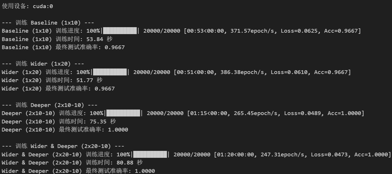
def train_and_evaluate_model(model_name, model_class, num_epochs=20000, lr=0.01, log_interval=200):print(f"\n--- 训练 {model_name} ---")model = model_class().to(device)criterion = nn.CrossEntropyLoss()optimizer = optim.SGD(model.parameters(), lr=lr)train_losses = []test_accuracies = []epochs_log = []start_time = time.time()with tqdm(total=num_epochs, desc=f"{model_name} 训练进度", unit="epoch") as pbar:for epoch in range(num_epochs):# 训练阶段model.train() # 设置为训练模式outputs = model(X_train)loss = criterion(outputs, y_train)optimizer.zero_grad()loss.backward()optimizer.step()# 评估阶段if (epoch + 1) % log_interval == 0:model.eval() # 设置为评估模式with torch.no_grad(): # 不计算梯度test_outputs = model(X_test)_, predicted = torch.max(test_outputs.data, 1)total = y_test.size(0)correct = (predicted == y_test).sum().item()accuracy = correct / totaltrain_losses.append(loss.item())test_accuracies.append(accuracy)epochs_log.append(epoch + 1)pbar.set_postfix({'Loss': f'{loss.item():.4f}', 'Acc': f'{accuracy:.4f}'})pbar.update(1) # 每次循环更新1步end_time = time.time()training_time = end_time - start_timeprint(f'{model_name} 训练时间: {training_time:.2f} 秒')# 最终评估model.eval()with torch.no_grad():test_outputs = model(X_test)_, predicted = torch.max(test_outputs.data, 1)total = y_test.size(0)correct = (predicted == y_test).sum().item()final_accuracy = correct / totalprint(f'{model_name} 最终测试准确率: {final_accuracy:.4f}')return {'model': model,'losses': train_losses,'accuracies': test_accuracies,'epochs': epochs_log,'time': training_time,'final_accuracy': final_accuracy}# 运行不同模型并收集结果
results = {}# Baseline MLP
results['Baseline (1x10)'] = train_and_evaluate_model('Baseline (1x10)', MLP_Baseline)# Wider MLP
results['Wider (1x20)'] = train_and_evaluate_model('Wider (1x20)', MLP_Wider)# Deeper MLP
results['Deeper (2x10-10)'] = train_and_evaluate_model('Deeper (2x10-10)', MLP_Deeper)# Wider & Deeper MLP
results['Wider & Deeper (2x20-10)'] = train_and_evaluate_model('Wider & Deeper (2x20-10)', MLP_WiderDeeper)# 可视化结果
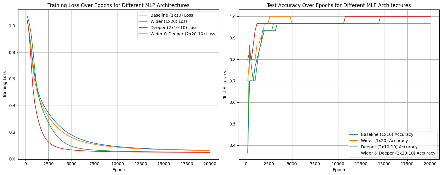
plt.figure(figsize=(15, 6))# 损失曲线
plt.subplot(1, 2, 1)
for name, res in results.items():plt.plot(res['epochs'], res['losses'], label=f'{name} Loss')
plt.xlabel('Epoch')
plt.ylabel('Training Loss')
plt.title('Training Loss Over Epochs for Different MLP Architectures')
plt.legend()
plt.grid(True)# 准确率曲线
plt.subplot(1, 2, 2)
for name, res in results.items():plt.plot(res['epochs'], res['accuracies'], label=f'{name} Accuracy')
plt.xlabel('Epoch')
plt.ylabel('Test Accuracy')
plt.title('Test Accuracy Over Epochs for Different MLP Architectures')
plt.legend()
plt.grid(True)plt.tight_layout()
plt.show()# 打印最终准确率和训练时间汇总
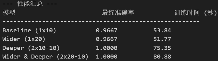
print("\n--- 性能汇总 ---")
print("{:<25} {:<15} {:<15}".format("模型", "最终准确率", "训练时间 (秒)"))
print("-" * 55)
for name, res in results.items():print("{:<25} {:<15.4f} {:<15.2f}".format(name, res['final_accuracy'], res['time']))