Matplotlib直线绘制:从基础到三维空间的高级可视化
在数据科学和工程领域,可视化是将抽象数据转化为直观洞察的关键桥梁。作为Python生态系统中最强大的绘图库之一,Matplotlib提供了从基础二维图形到复杂三维可视化的全面工具集。直线作为最基本的几何元素,其绘制方法贯穿于数据可视化的各个领域。本文将深入探讨Matplotlib中直线绘制的核心技术与应用实践,帮助读者掌握从基础到高级的直线可视化方法。
使用Matplotlib绘制直线(已知起点和终点)
在Matplotlib中,你可以使用plot()函数或Line2D对象来绘制直线。以下是几种方法:
方法1:使用plot()函数
import matplotlib.pyplot as plt# 定义起点和终点坐标
start_point = (1, 2)  # (x1, y1)
end_point = (5, 8)    # (x2, y2)# 绘制直线
plt.plot([start_point[0], end_point[0]], [start_point[1], end_point[1]], color='blue', linewidth=2, linestyle='-')# 设置坐标轴范围
plt.xlim(0, 10)
plt.ylim(0, 10)# 显示图形
plt.show()
方法2:使用Line2D对象
import matplotlib.pyplot as plt
from matplotlib.lines import Line2D# 创建图形和坐标轴
fig, ax = plt.subplots()# 定义起点和终点
start = (3, 4)
end = (7, 6)# 创建Line2D对象
line = Line2D([start[0], end[0]], [start[1], end[1]], color='red', linewidth=3, linestyle='--')# 添加到坐标轴
ax.add_line(line)# 设置坐标轴范围
ax.set_xlim(0, 10)
ax.set_ylim(0, 10)# 显示图形
plt.show()
方法3:使用annotate绘制带箭头的直线
import matplotlib.pyplot as plt# 定义起点和终点
start = (2, 3)
end = (8, 7)# 绘制带箭头的直线
plt.annotate('', xy=end, xytext=start,arrowprops=dict(arrowstyle='->', linewidth=2, color='green'))# 设置坐标轴范围
plt.xlim(0, 10)
plt.ylim(0, 10)# 显示图形
plt.show()
绘制多组起点-终点的直线(使用数组存储坐标)
如果起点和终点的x、y坐标分别存储在四个一维数组Sx、Sy、Ex、Ey中,你可以使用以下几种方法绘制多组直线:
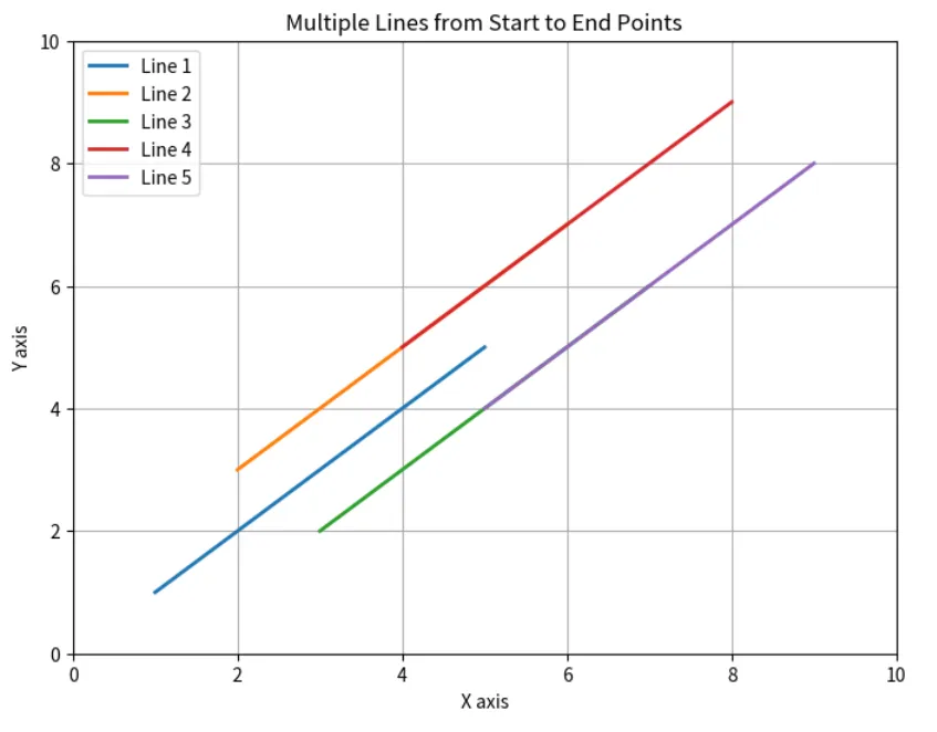
方法1:使用循环逐条绘制
import matplotlib.pyplot as plt# 示例数据 - 假设有5条直线
Sx = [1, 2, 3, 4, 5]  # 起点x坐标
Sy = [1, 3, 2, 5, 4]  # 起点y坐标
Ex = [5, 6, 7, 8, 9]  # 终点x坐标
Ey = [5, 7, 6, 9, 8]  # 终点y坐标# 创建图形
plt.figure(figsize=(8, 6))# 循环绘制每条直线
for i in range(len(Sx)):plt.plot([Sx[i], Ex[i]], [Sy[i], Ey[i]], linewidth=2, label=f'Line {i+1}')# 添加图例
plt.legend()# 设置坐标轴范围
plt.xlim(0, 10)
plt.ylim(0, 10)# 添加标题和标签
plt.title('Multiple Lines from Start to End Points')
plt.xlabel('X axis')
plt.ylabel('Y axis')# 显示图形
plt.grid(True)
plt.show()
方法2:使用向量化操作(更高效)
import matplotlib.pyplot as plt
import numpy as np# 示例数据转换为numpy数组
Sx = np.array([1, 2, 3, 4, 5])
Sy = np.array([1, 3, 2, 5, 4])
Ex = np.array([5, 6, 7, 8, 9])
Ey = np.array([5, 7, 6, 9, 8])# 创建图形
plt.figure(figsize=(8, 6))# 向量化绘制 - 更高效
plt.plot(np.vstack([Sx, Ex]), np.vstack([Sy, Ey]), linewidth=2)# 添加起点和终点标记
plt.scatter(Sx, Sy, c='red', s=100, label='Start Points')
plt.scatter(Ex, Ey, c='blue', s=100, label='End Points')# 设置坐标轴范围
plt.xlim(0, 10)
plt.ylim(0, 10)# 添加图例和标题
plt.legend()
plt.title('Vectorized Line Drawing')
plt.xlabel('X axis')
plt.ylabel('Y axis')# 显示图形
plt.grid(True)
plt.show()
方法3:使用LineCollection(适合大量直线)
import matplotlib.pyplot as plt
from matplotlib.collections import LineCollection
import numpy as np# 示例数据
Sx = np.array([1, 2, 3, 4, 5])
Sy = np.array([1, 3, 2, 5, 4])
Ex = np.array([5, 6, 7, 8, 9])
Ey = np.array([5, 7, 6, 9, 8])# 准备线段数据 - 每条线段由起点和终点组成
segments = np.array([[[sx, sy], [ex, ey]] for sx, sy, ex, ey in zip(Sx, Sy, Ex, Ey)])# 创建LineCollection
line_collection = LineCollection(segments, linewidths=2,colors=['red', 'green', 'blue', 'purple', 'orange'],linestyle='solid')# 创建图形
fig, ax = plt.subplots(figsize=(8, 6))# 添加线段集合
ax.add_collection(line_collection)# 设置坐标轴范围
ax.set_xlim(0, 10)
ax.set_ylim(0, 10)# 添加标记和标题
ax.scatter(Sx, Sy, c='red', s=100, label='Start Points')
ax.scatter(Ex, Ey, c='blue', s=100, label='End Points')
ax.set_title('LineCollection Example')
ax.legend()# 显示图形
plt.grid(True)
plt.show()
在Matplotlib中绘制三维空间直线(已知起点和终点)
在三维空间中绘制直线,Matplotlib的mplot3d工具包提供了相应的功能。以下是几种方法来绘制三维直线,假设起点和终点的坐标分别存储在数组Sx, Sy, Sz和Ex, Ey, Ez中。
方法1:使用Axes3D的plot()函数逐条绘制
import matplotlib.pyplot as plt
from mpl_toolkits.mplot3d import Axes3D
import numpy as np# 创建示例数据(5条直线)
Sx = np.array([1, 2, 3, 4, 5])  # 起点x坐标
Sy = np.array([1, 3, 2, 5, 4])  # 起点y坐标
Sz = np.array([0, 1, 2, 1, 3])  # 起点z坐标
Ex = np.array([5, 6, 7, 8, 9])  # 终点x坐标
Ey = np.array([5, 7, 6, 9, 8])  # 终点y坐标
Ez = np.array([5, 6, 7, 8, 9])  # 终点z坐标# 创建3D图形
fig = plt.figure(figsize=(10, 8))
ax = fig.add_subplot(111, projection='3d')# 循环绘制每条直线
for i in range(len(Sx)):ax.plot([Sx[i], Ex[i]], [Sy[i], Ey[i]], [Sz[i], Ez[i]],linewidth=2,label=f'Line {i+1}')# 添加起点和终点标记
ax.scatter(Sx, Sy, Sz, c='red', s=100, label='Start Points')
ax.scatter(Ex, Ey, Ez, c='blue', s=100, label='End Points')# 设置坐标轴标签
ax.set_xlabel('X Axis')
ax.set_ylabel('Y Axis')
ax.set_zlabel('Z Axis')# 设置坐标轴范围
ax.set_xlim(0, 10)
ax.set_ylim(0, 10)
ax.set_zlim(0, 10)# 添加图例和标题
ax.legend()
plt.title('3D Lines from Start to End Points')# 显示图形
plt.show()
方法2:使用向量化操作绘制(更高效)
import matplotlib.pyplot as plt
from mpl_toolkits.mplot3d import Axes3D
import numpy as np# 示例数据
Sx = np.array([1, 2, 3, 4, 5])
Sy = np.array([1, 3, 2, 5, 4])
Sz = np.array([0, 1, 2, 1, 3])
Ex = np.array([5, 6, 7, 8, 9])
Ey = np.array([5, 7, 6, 9, 8])
Ez = np.array([5, 6, 7, 8, 9])# 创建3D图形
fig = plt.figure(figsize=(10, 8))
ax = fig.add_subplot(111, projection='3d')# 准备线段数据
x_lines = np.vstack([Sx, Ex]).T
y_lines = np.vstack([Sy, Ey]).T
z_lines = np.vstack([Sz, Ez]).T# 向量化绘制
for x, y, z in zip(x_lines, y_lines, z_lines):ax.plot(x, y, z, linewidth=2)# 添加标记
ax.scatter(Sx, Sy, Sz, c='red', s=100, label='Start Points')
ax.scatter(Ex, Ey, Ez, c='blue', s=100, label='End Points')# 设置图形属性
ax.set_xlabel('X Axis')
ax.set_ylabel('Y Axis')
ax.set_zlabel('Z Axis')
ax.set_xlim(0, 10)
ax.set_ylim(0, 10)
ax.set_zlim(0, 10)
ax.legend()
plt.title('Vectorized 3D Line Drawing')plt.show()
方法3:使用Line3DCollection(适合大量直线)
import matplotlib.pyplot as plt
from mpl_toolkits.mplot3d import Axes3D
from mpl_toolkits.mplot3d.art3d import Line3DCollection
import numpy as np# 示例数据
Sx = np.array([1, 2, 3, 4, 5])
Sy = np.array([1, 3, 2, 5, 4])
Sz = np.array([0, 1, 2, 1, 3])
Ex = np.array([5, 6, 7, 8, 9])
Ey = np.array([5, 7, 6, 9, 8])
Ez = np.array([5, 6, 7, 8, 9])# 准备线段数据
segments = np.array([[[sx, sy, sz], [ex, ey, ez]] for sx, sy, sz, ex, ey, ez in zip(Sx, Sy, Sz, Ex, Ey, Ez)])# 创建3D图形
fig = plt.figure(figsize=(10, 8))
ax = fig.add_subplot(111, projection='3d')# 创建Line3DCollection
line_collection = Line3DCollection(segments, linewidths=2,colors=['red', 'green', 'blue', 'purple', 'orange'])# 添加到图形
ax.add_collection3d(line_collection)# 添加标记
ax.scatter(Sx, Sy, Sz, c='red', s=100, label='Start Points')
ax.scatter(Ex, Ey, Ez, c='blue', s=100, label='End Points')# 设置图形属性
ax.set_xlabel('X Axis')
ax.set_ylabel('Y Axis')
ax.set_zlabel('Z Axis')
ax.set_xlim(0, 10)
ax.set_ylim(0, 10)
ax.set_zlim(0, 10)
ax.legend()
plt.title('3D Line Collection')plt.show()
高级技巧:添加箭头和标签
import matplotlib.pyplot as plt
from mpl_toolkits.mplot3d import Axes3D
import numpy as np# 示例数据
Sx = np.array([1, 3, 5])
Sy = np.array([1, 3, 5])
Sz = np.array([0, 2, 4])
Ex = np.array([5, 7, 9])
Ey = np.array([5, 7, 9])
Ez = np.array([5, 7, 9])# 创建3D图形
fig = plt.figure(figsize=(10, 8))
ax = fig.add_subplot(111, projection='3d')# 绘制带箭头的直线
for i in range(len(Sx)):# 绘制直线ax.plot([Sx[i], Ex[i]], [Sy[i], Ey[i]], [Sz[i], Ez[i]],linewidth=2,label=f'Line {i+1}')# 添加箭头ax.quiver(Sx[i], Sy[i], Sz[i], Ex[i]-Sx[i], Ey[i]-Sy[i], Ez[i]-Sz[i],arrow_length_ratio=0.1, color='red')# 设置图形属性
ax.set_xlabel('X Axis')
ax.set_ylabel('Y Axis')
ax.set_zlabel('Z Axis')
ax.set_xlim(0, 10)
ax.set_ylim(0, 10)
ax.set_zlim(0, 10)
ax.legend()
plt.title('3D Lines with Arrows')plt.show()
这些方法可以灵活应用于各种三维数据可视化场景,如分子结构、空间轨迹、三维向量场等。