python时间序列处理
(1)numpy 中的时间序列
时间类型:numpy.datetime64
创建时间类型变量
import numpy as npx = np.datetime64('2018-12-16')
print(type(x))  #  <class 'numpy.datetime64'>
print(x)           # 2018-12-16
设置时间型数值的精度
Y 年 M 月 W 周 D 日 h 时 m 分 s 秒
ms 毫秒 us 微秒 ns 纳秒 ps 皮秒 fs 飞秒 as 原秒
import numpy as np# 不设定精度的话就是输入值的精度
print(np.datetime64('2018-12-16 10:31'))
# 2018-12-16T10:31 # 设置精度到秒
print(np.datetime64('2018-12-16', "s"))
# 2018-12-16T00:00:00# 设置精度在毫秒
print(np.datetime64('2018-12-16 12:59:59.50', 'ms'))
# 2018-12-16T12:59:59.500 # 精度到秒,小数部分自动砍掉
print(np.datetime64('2018-12-16 12:59:59.577', 's'))
# 2018-12-16T12:59:59
创建时间型序列,类型用np.datetime64
import numpy as np# 唯一类型 datetime64
date = np.array('2018-12-16', dtype = np.datetime64)
print(type(date)) # <class 'numpy.ndarray'>
print(date)       # 2018-12-16data = ['2018-12-16', '2018-12-17', '2018-12-18']
date = np.array(data, dtype = np.datetime64)
print(type(date)) # <class 'numpy.ndarray'>
print(date)       # ['2018-12-16' '2018-12-17' '2018-12-18']# 快速生成等步长的时间序列数据
date = np.array('2018-12-16', dtype = np.datetime64)
delta = np.arange(30)
print(date + delta)
'''
['2018-12-16' '2018-12-17' '2018-12-18' '2018-12-19' '2018-12-20''2018-12-21' '2018-12-22' '2018-12-23' '2018-12-24' '2018-12-25''2018-12-26' '2018-12-27' '2018-12-28' '2018-12-29' '2018-12-30''2018-12-31' '2019-01-01' '2019-01-02' '2019-01-03' '2019-01-04''2019-01-05' '2019-01-06' '2019-01-07' '2019-01-08' '2019-01-09''2019-01-10' '2019-01-11' '2019-01-12' '2019-01-13' '2019-01-14']
'''
(2)Pandas中的时间序列
以下将会提到四种时间类型:
- 时间戳:表示一个时间点,类型为Timestamp
- 时间增量:两个时间的差,类型为Timedelta
- 时间周期:表示一段时间,类型为Period
- 时间字符串:带时间信息的字符串,类型为str
1.时间戳 Timestamp
①pd.DatetimeIndex():创建时间戳类型的 index
下面是一个例子,创建一个index类型为时间戳序列的df
timeindex = pd.DatetimeIndex(['2014-07-04', '2014-08-04','2015-07-04', '2015-08-04'])
data = pd.Series([3, 1, 5, 4], index = timeindex)
print(data)
# 2014-07-04    3
# 2014-08-04    1
# 2015-07-04    5
# 2015-08-04    4
# dtype: int64print(data['2014-07-04':'2015-07-04'])
# 2014-07-04    3
# 2014-08-04    1
# 2015-07-04    5
# dtype: int64
②时间戳类型index的妙用
timeindex = pd.DatetimeIndex(['2014-07-04', '2014-08-04','2015-07-04', '2015-08-04'])
data = pd.Series([3, 1, 5, 4], index = timeindex)print("特殊取法:根据时间索引值的部分索引")
print(data['2015'])
# 2015-07-04    5
# 2015-08-04    4
# dtype: int64print(data['2015-07'])
# 2015-07-04    5
# dtype: int64③pd.to_datetime():将时间字符串转化为时间戳
Pandas 所有关于日期与时间的处理方法全部都是通过 Timestamp 对象实现的。它利用 numpy.datetime64 的有效存储和向量化接口将 datetime 和 dateutil 的易用性有机结合起来。
import pandas as pd
import numpy as np
from datetime import datetimedate = pd.to_datetime("17th of December, 2018")
print(type(date)) # <class 'pandas._libs.tslibs.timestamps.Timestamp'>
print(date) # 2018-12-17 00:00:00print(pd.to_datetime('2015-Jul-6'))
# 2015-07-06 00:00:00print(pd.to_datetime(['2015-Jul-6', '2015-Jul-6'])) # DatetimeIndex
# DatetimeIndex(['2015-07-06', '2015-07-06'], dtype='datetime64[ns]', freq=None)dates = pd.to_datetime([datetime(2015, 7, 3), '4th of July, 2015','2015-Jul-6', '07-07-2015', '20150708'])
print(dates)
# DatetimeIndex(['2015-07-03', '2015-07-04', '2015-07-06', '2015-07-07',
#                '2015-07-08'],
#               dtype='datetime64[ns]', freq=None)
④datetime.strftime():将时间戳转化为时间字符串
date = pd.to_datetime("17th of December, 2018")
print(date) # 2018-12-17 00:00:00
print(date.strftime('%A')) # Monday
print(date.strftime('%Y-%m-%d')) # 2018-12-17
print(date.strftime('%Y#%m#%d')) # 2018#12#17
关于不同格式的含义可以参考这篇文章结尾那里:python中的时间模块-CSDN博客
2.时间增量 timedelta
①pd.to_timedelta(序列对象, 时间单位):生成时间增量
第二个参数时间单位是用来设置精度的,前面numpy时间序列那里有讲过。
import pandas as pd
import numpy as npdelta1 = pd.to_timedelta(np.arange(12), 'D')
delta2 = pd.to_timedelta([1, 2, 3, 4], 'D')
print(delta1)
# TimedeltaIndex([ '0 days',  '1 days',  '2 days',  '3 days',  '4 days',
#                  '5 days',  '6 days',  '7 days',  '8 days',  '9 days',
#                 '10 days', '11 days'],
#                dtype='timedelta64[ns]', freq=None)print(delta2)
# TimedeltaIndex(['1 days', '2 days', '3 days', '4 days'], dtype='timedelta64[ns]', freq=None)
②用"时间戳+时间增量"生成多个时间戳
date = pd.to_datetime("17th of December, 2018")
delta = pd.to_timedelta(np.arange(12), 'D')
print(date + delta)# DatetimeIndex(['2018-12-17', '2018-12-18', '2018-12-19', '2018-12-20',
#                '2018-12-21', '2018-12-22', '2018-12-23', '2018-12-24',
#                '2018-12-25', '2018-12-26', '2018-12-27', '2018-12-28'],
#               dtype='datetime64[ns]', freq=None)
③通过两个时间戳相减得到时间增量
dates = pd.to_datetime([datetime(2015, 7, 3), '4th of July, 2015','2015-Jul-6', '07-07-2015', '20150708'])
print(dates)
# DatetimeIndex(['2015-07-03', '2015-07-04', '2015-07-06', '2015-07-07',
#                '2015-07-08'],
#               dtype='datetime64[ns]', freq=None)print(dates[0])
# 2015-07-03 00:00:00print(dates - dates[0])
# TimedeltaIndex(['0 days', '1 days', '3 days', '4 days', '5 days'], dtype='timedelta64[ns]', freq=None)
3.一段时期 Period
Period:时间周期,表示一段时期
①pd.Period():时间戳变为时间周期
import pandas as pdprint("\n①不指定频率时,则默认用当前精度这段时间")
print("比如下面2021就表示2021年年初到2021年年末")
year = pd.Period('2021')
print( 'Start Time:', year.start_time) # 2021-01-01 00:00:00
print( 'End Time:', year.end_time) # 2021-12-31 23:59:59.999999999print("\n再比如2021-02就表示2021年2月月初到2021年2月月末")
year = pd.Period('2021-02')
print( 'Start Time:', year.start_time) # 2021-01-01 00:00:00
print( 'End Time:', year.end_time) # 2021-12-31 23:59:59.999999999print("\n②使用 freq 参数显式指定周期的频率")
print("这里用天,就表示一天的时期")
print("自动变为所给日期的当天,若未给天的日期,则为当月 1 号")
day = pd.Period( '2022-01', freq= 'D')
print( 'Start Time:', day.start_time) # 2022-01-01 00:00:00
print( 'End Time:', day.end_time) # 2022-01-01 23:59:59.999999999day = pd.Period( '2022-01-02', freq= 'D')
print( 'Start Time:', day.start_time) # 2022-01-02 00:00:00
print( 'End Time:', day.end_time) # 2022-01-02 23:59:59.999999999
②to_period():将时间戳序列变为时间周期序列
import pandas as pd
import numpy as np
from datetime import datetimedates = pd.to_datetime([datetime(2015, 7, 3), '4th of July, 2015', '2015-Jul-6', '07-07-2015', '20150708'])
print(dates)
print(type(dates[0]))   # 时间戳 Timestampper_arr = dates.to_period('M')
print(per_arr)
# PeriodIndex(['2015-07', '2015-07', '2015-07', '2015-07', '2015-07'], dtype='period[M]', freq='M')
print(type(per_arr[0]))  # 时间周期 Period
print(per_arr[0])
print(per_arr[0].start_time)
print(per_arr[0].end_time)
③时间周期与标量进行运算,得到新的时间周期
hour = pd.Period( '2022-02-09 16:00:00', freq= 'H')
x = hour + 2
y = hour - 2
print(type(x))  # <class 'pandas._libs.tslibs.period.Period'>
print(x)   #  2022-02-09 18:00
print(y)   #  2022-02-09 14:00delta = np.arange(10)
result = hour + delta
print(type(result))  # <class 'numpy.ndarray'>
print(result)
# [Period('2022-02-09 16:00', 'H') Period('2022-02-09 17:00', 'H')
#  Period('2022-02-09 18:00', 'H') Period('2022-02-09 19:00', 'H')
#  Period('2022-02-09 20:00', 'H') Period('2022-02-09 21:00', 'H')
#  Period('2022-02-09 22:00', 'H') Period('2022-02-09 23:00', 'H')
#  Period('2022-02-10 00:00', 'H') Period('2022-02-10 01:00', 'H')]
4.批量生成多个时间戳/时间周期/时间增量
pd.date_range()
例子1:生成多个天的日期序列
# help(pd.date_range)
# date_range(start=None, end=None, periods=None, freq=None, tz=None, normalize=False, name=None, closed=None)print(pd.date_range('2015-07-03', '2015-07-10'))
# DatetimeIndex(['2015-07-03', '2015-07-04', '2015-07-05', '2015-07-06',
#                '2015-07-07', '2015-07-08', '2015-07-09', '2015-07-10'],
#               dtype='datetime64[ns]', freq='D')print(pd.date_range('2015-07-03', periods = 8))
# DatetimeIndex(['2015-07-03', '2015-07-04', '2015-07-05', '2015-07-06',
#                '2015-07-07', '2015-07-08', '2015-07-09', '2015-07-10'],
#               dtype='datetime64[ns]', freq='D')print(pd.date_range('2015-07-03', periods = 8, freq = 'H'))
# DatetimeIndex(['2015-07-03 00:00:00', '2015-07-03 01:00:00',
#                '2015-07-03 02:00:00', '2015-07-03 03:00:00',
#                '2015-07-03 04:00:00', '2015-07-03 05:00:00',
#                '2015-07-03 06:00:00', '2015-07-03 07:00:00'],
#               dtype='datetime64[ns]', freq='H')
例子2:生成多个年末最后一天的时间序列
import pandas as pd
from pandas.tseries.offsets import *dates = pd.date_range('2015-07-01', periods=10, freq = BYearEnd())
# freq参数 按年末(最后一个工作日)生成多个时间戳
print(dates)
# DatetimeIndex(['2015-12-31', '2016-12-30', '2017-12-29', '2018-12-31',
#                '2019-12-31', '2020-12-31', '2021-12-31', '2022-12-30',
#                '2023-12-29', '2024-12-31'],
#               dtype='datetime64[ns]', freq='BA-DEC')
pd.period_range()
例子:生成多个季节周期
# period_range(start=None, end=None, periods=None, freq=None, name=None)
print(pd.period_range('2015-07', periods = 8, freq = 'Q'))# PeriodIndex(['2015Q3', '2015Q4', '2016Q1', '2016Q2', '2016Q3', '2016Q4',
#              '2017Q1', '2017Q2'],
#             dtype='period[Q-DEC]', freq='Q-DEC')
pd.timedelta_range()
例子:生成按小时递增的时间增量
# timedelta_range(start=None, end=None, periods=None, freq=None, name=None, closed=None)print(pd.timedelta_range(0, periods=24, freq='H'))
# TimedeltaIndex(['00:00:00', '01:00:00', '02:00:00', '03:00:00', '04:00:00',
#                 '05:00:00', '06:00:00', '07:00:00', '08:00:00', '09:00:00',
#                 '10:00:00', '11:00:00', '12:00:00', '13:00:00', '14:00:00',
#                 '15:00:00', '16:00:00', '17:00:00', '18:00:00', '19:00:00',
#                 '20:00:00', '21:00:00', '22:00:00', '23:00:00'],
#                dtype='timedelta64[ns]', freq='H')
5.时间频率参数 freq
查看所有的频率类型
import pandas as pd
from pandas.tseries.offsets import *for offset in dir(pd.tseries.offsets):print(offset)
频率解释
例子使用理解
print(pd.timedelta_range(0, periods = 20, freq = "2H30T")) # 时间频率为 2 小时 30 分钟
# TimedeltaIndex(['0 days 00:00:00', '0 days 02:30:00', '0 days 05:00:00',
#                 '0 days 07:30:00', '0 days 10:00:00', '0 days 12:30:00',
#                 '0 days 15:00:00', '0 days 17:30:00', '0 days 20:00:00',
#                 '0 days 22:30:00', '1 days 01:00:00', '1 days 03:30:00',
#                 '1 days 06:00:00', '1 days 08:30:00', '1 days 11:00:00',
#                 '1 days 13:30:00', '1 days 16:00:00', '1 days 18:30:00',
#                 '1 days 21:00:00', '1 days 23:30:00'],
#                dtype='timedelta64[ns]', freq='150T')print(pd.date_range('2015-07-03', periods = 8, freq = 'BA'))
# DatetimeIndex(['2015-12-31', '2016-12-30', '2017-12-29', '2018-12-31',
#                '2019-12-31', '2020-12-31', '2021-12-31', '2022-12-30'],
#               dtype='datetime64[ns]', freq='BA-DEC')
6.时间分组 df.resample()和 df.asfreq()
这两个方法都是对时间序列进行分组,比如我们有12天的12条数据,现在我们按3天一组,就可以得到4组数据,然后对每个组进行统计啥的。
那这个两个方法的区别是啥,
- resample() : 将每个组的全部数据取出来
- asfreq() : 只取每个组的端点时间
例子1:resample()使用
import pandas as pd
import numpy as np# 生成时间索引,频率T是分钟
ts_index = pd.date_range('2018-08-03', periods=12, freq='T')
ts = pd.Series(np.arange(12), index=ts_index)
print("\n", ts)
'''
2018-08-03 00:00:00     0
2018-08-03 00:01:00     1
2018-08-03 00:02:00     2
2018-08-03 00:03:00     3
2018-08-03 00:04:00     4
2018-08-03 00:05:00     5
2018-08-03 00:06:00     6
2018-08-03 00:07:00     7
2018-08-03 00:08:00     8
2018-08-03 00:09:00     9
2018-08-03 00:10:00    10
2018-08-03 00:11:00    11
Freq: T, dtype: int32
'''# print("\n", ts.resample('5min'))# 按5分钟级别进行时间分组,然后对每个组求和
# 区间默认是左闭右开,比如这里前5分钟是[00:00:00, 00:05:00)
print("\n", ts.resample('5min').sum())
'''
2018-08-03 00:00:00    10
2018-08-03 00:05:00    35
2018-08-03 00:10:00    21
Freq: 5T, dtype: int32
'''# 使用参数closed='right’可以使得区间右端也可以取到
print("\n", ts.resample('5min', closed='right').sum())
'''
2018-08-02 23:55:00     0
2018-08-03 00:00:00    15
2018-08-03 00:05:00    40
2018-08-03 00:10:00    11
Freq: 5T, dtype: int32
'''
例子2:asfreq()使用
print(ts.asfreq('5min'))'''
2018-08-03 00:00:00     0
2018-08-03 00:05:00     5
2018-08-03 00:10:00    10
Freq: 5T, dtype: int32
'''#help(ts.asfreq)
例子3:股票数据处理
①加载数据
import pandas as pd
import tushare as ts%matplotlib inline
import matplotlib.pyplot as plt
import seaborn; seaborn.set()# 获取某只股票的交易数据(DataFrame)
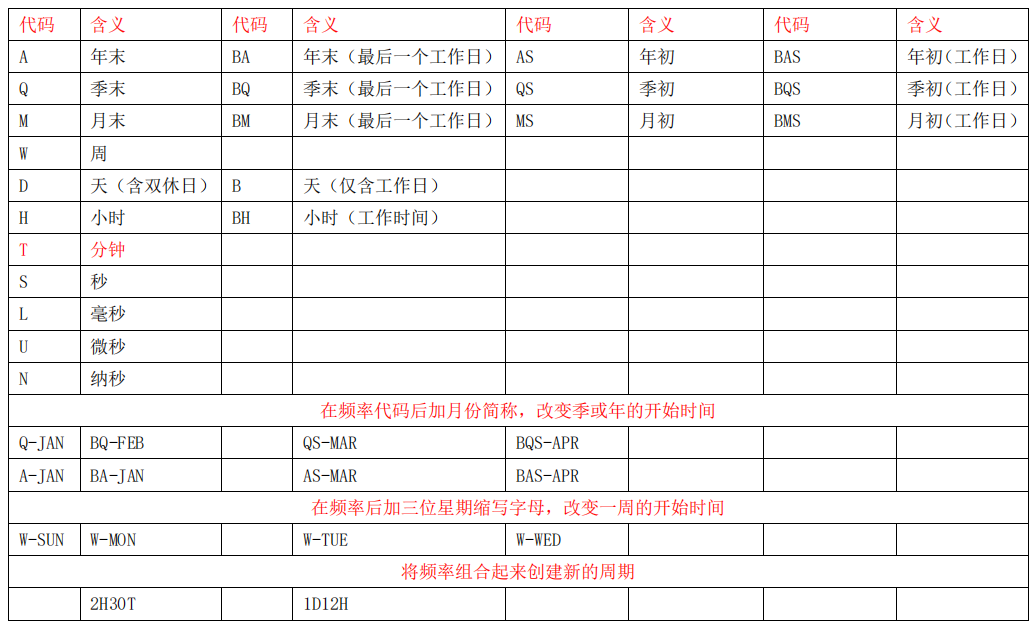
stock = ts.get_k_data(code='600547',start='2020', end='2023')
#本接口即将停止更新,请尽快使用Pro版接口:https://waditu.com/document/2
print(stock.head())
# date open close high low volume code
# 0 2020-01-02 22.907 23.329 23.371 22.871 489106.0 600547
# 1 2020-01-03 23.550 24.671 25.007 23.471 987248.0 600547
# 2 2020-01-06 25.900 26.907 26.950 25.900 1234004.0 600547
# 3 2020-01-07 26.107 26.086 26.307 25.550 707042.0 600547
# 4 2020-01-08 27.693 27.321 27.886 26.350 1326357.0 600547# 将'date'列的数据格式转化为时间戳格式
stock['date'] = pd.to_datetime(stock['date']) # 将 date 列变为行索引
stock.set_index('date', inplace=True) # 数据只要收盘价这一列
stock = stock['close'] # 画图
plt.plot(stock)
plt.show()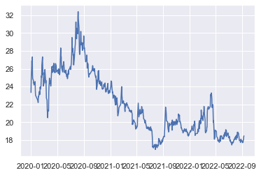
②对年内所有天平均,以及年末最后一天的值
print(list(stock.resample('BA')))
# BA 表示年末(最后一个工作日),这里就是年末到年末之间为一个时间段(一个组)
# 该列表的每个元素是 series,每个 series 表示某一年所有天的数据print(stock.asfreq('BA'))
# 只取了时间段的端点值,这里时间段是年末到年末,所以取的都是年末的值
# date
# 2020-12-31    23.52
# 2021-12-31    18.77
# Freq: BA-DEC, Name: close, dtype: float64# alpha 表示透明度,越接近 0 越透明,越接近 1 越不透明
stock.plot(alpha = 0.5, style = '-') # 统计每一年内的平均值
stock.resample('BA').mean().plot(style = ':') # 统计年末最后一天的值
stock.asfreq('BA').plot(style = '--')# 图例设置
plt.legend(['input', 'resample', 'asfreq'], loc = 'upper center')
plt.show()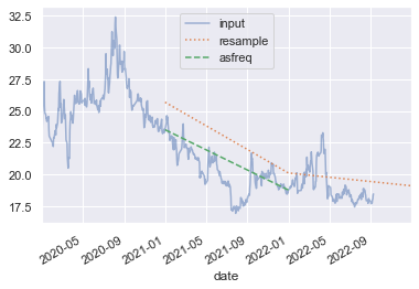
③将缺失值填充为指定值
print(stock.iloc[:10]) # 查看前 10 行可以发现缺失部分日期
'''
date
2020-01-02    23.329
2020-01-03    24.671
2020-01-06    26.907
2020-01-07    26.086
2020-01-08    27.321
2020-01-09    25.350
2020-01-10    24.871
2020-01-13    24.693
2020-01-14    24.393
2020-01-15    24.443
Name: close, dtype: float64
'''# (2,1):2 行 1 列个图形
fig, ax = plt.subplots(2, sharex = True)
data = stock.iloc[:10]# 不填充缺失值画图
data.asfreq('D').plot(ax = ax[0], marker = 'o')# 后向填充缺失值(缺失数据用明天的数据填充)
data.asfreq('D', method = 'bfill').plot(ax = ax[1], style = '-o') # 前向填充缺失值(缺失数据用前一天填充)
data.asfreq('D', method = 'ffill').plot(ax = ax[1], style = '--o')
ax[1].legend(["back-fill", "forward-fill"])
plt.show()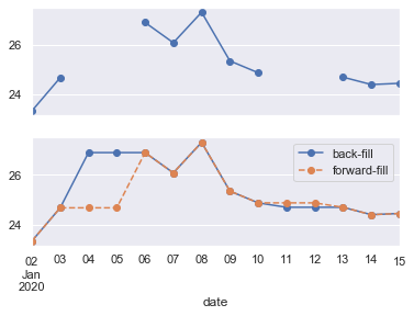
7.日期平移和数据平移
datetimeSeries.shift():平移数据
datetimeSeries.tshift():平移索引
平移什么意思?比如我们长度为3的时间序列数据,比如下面这样
日期         值
20250101    100
20250102    5
20250103    31
现在我们将日期这一列平移一天,同时值这一列不动,就变成了这样
日期         值
20250102    100
20250103    5
20250104    31
这就是对日期进行平移。
平移有什么用?明显做差分可以用到,当然也还有其它用处,算移动平均啥的。
例子1:用法示例
import pandas as pd
import tushare as ts# % matplotlib inline
import matplotlib.pyplot as plt
import seabornseaborn.set()# 获取某只股票的交易数据(DataFrame)
stock = ts.get_k_data(code='600547', start='2018', end='2023')# 将date列的数据格式转化为时间戳格式
stock['date'] = pd.to_datetime(stock['date'])# 将 date 列变为行索引
stock.set_index('date', inplace=True)# 只取收盘价
stock = stock['close']# 准备3个子图画图,(3,1)个图形 # 共享 y 轴
fig, ax = plt.subplots(3, sharey=True)  #
fig.subplots_adjust(hspace=0.4, wspace=0.4)# 对数据应用时间频率,pad 也表示前向填充
stock = stock.asfreq('D', method='pad')  # 画图两种方式:ax[0].plot(x,y) data.plot(ax = ax[0])
stock.plot(ax=ax[0])  # 平移数据
stock.shift(900).plot(ax=ax[1])  # 平移索引
stock.tshift(900).plot(ax=ax[2])  # 设置图例与标签
local_max = pd.to_datetime('2021-01-01')
offset = pd.Timedelta(900, 'D')ax[0].legend(['input'], loc=2)
# 将 x 轴第 4 个标签值加粗,红色
ax[0].get_xticklabels()[3].set(weight='heavy', color='red')
# 画垂直的竖线 第一个参数是 x = 某个 xlabel
ax[0].axvline(local_max, alpha=0.3, color='red') ax[1].legend(['shift(900)'], loc=2)
ax[1].get_xticklabels()[3].set(weight='heavy', color='red')
ax[1].axvline(local_max + offset, alpha=0.3, color='red')ax[2].legend(['tshift(900)'], loc=2)
ax[2].get_xticklabels()[1].set(weight='heavy', color='red')
ax[2].axvline(local_max + offset, alpha=0.3, color='red')plt.show()   # 显示图像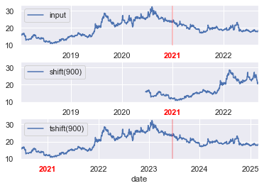
例子2:计算投资回报率
ROI = 100 * (stock.tshift(-365) / stock - 1)
# 比值是明年与今年同期比较
# 横坐标为今年
ROI.plot()
plt.ylabel('% Return on Investment')
plt.axhline(y = 0, c = 'r', ls = '--', lw = 2) # 设置水平参考线 # 注意结尾这个分号的作用
plt.show()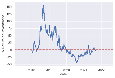
8.移动分组与统计
datetimeSeries.rolling(days, center = True):移动分组,比如可以移动分组后对每组求平均,就得到了移动平均
- 无 center 参数时,取前 days 天的数据为轴 0 的一个组;前面数据量小于 days 的,为空
- 有 center 时,以当前位置为中心,向左右平均取共 days 个数据的平均
例子
print(stock.head(10))  # # 可以看到是从 2018-01-02 开始的
'''
date
2018-01-02    15.818
2018-01-03    15.854
2018-01-04    15.824
2018-01-05    16.022
2018-01-06    16.022
2018-01-07    16.022
2018-01-08    16.237
2018-01-09    15.987
2018-01-10    15.660
2018-01-11    15.829
Freq: D, Name: close, dtype: float64
'''# 移动分组
rolling = stock.rolling(5)
# print(rolling) # Rolling [window=5,center=False,axis=0]
print(rolling.mean()[:10])
'''
date
2018-01-02        NaN
2018-01-03        NaN
2018-01-04        NaN
2018-01-05        NaN
2018-01-06    15.9080
2018-01-07    15.9488
2018-01-08    16.0254
2018-01-09    16.0580
2018-01-10    15.9856
2018-01-11    15.9470
Freq: D, Name: close, dtype: float64
'''rolling = stock.rolling(5, center=True)
print(rolling.mean()[:10])
'''
date
2018-01-02        NaN
2018-01-03        NaN
2018-01-04    15.9080
2018-01-05    15.9488
2018-01-06    16.0254
2018-01-07    16.0580
2018-01-08    15.9856
2018-01-09    15.9470
2018-01-10    16.0114
2018-01-11    16.0328
Freq: D, Name: close, dtype: float64
'''# rolling.mean()和 rolling.std()
rolling = stock.rolling(365, center=True)
data = pd.DataFrame({'input': stock,'one-year rolling_mean': rolling.mean(),'one-year rolling_std': rolling.std()})
ax = data.plot(style=['-', '--', ':'])
ax.lines[0].set_alpha(0.3)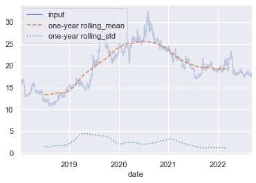
end