当前位置：首页 > news >正文

《Python星球日记》第63天：文本方向综合项目（新闻分类）

news 2025/5/13 6:07:38

名人说：路漫漫其修远兮，吾将上下而求索。—— 屈原《离骚》
创作者：Code_流苏(CSDN)（一个喜欢古诗词和编程的Coder😊）

目录

一、项目需求分析
1. 项目背景与目标
2. 功能需求
3. 技术方案概述

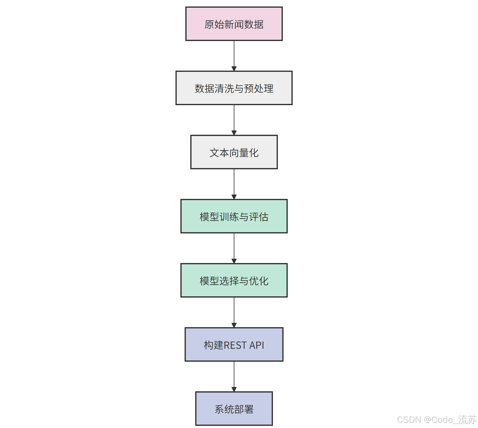
二、数据清洗与文本预处理
1. 数据集介绍
2. 数据清洗步骤
3. 文本向量化

三、模型选择与训练
1. RNN模型
2. LSTM模型
3. Transformer模型
4. 模型比较与选择

四、结果可视化与评估
1. 类别分布与预测置信度
2. 错误分析
3. 词云可视化

五、模型部署与API构建
1. 构建RESTful API
2. 保存和加载组件
3. 部署建议
4. 使用示例

六、项目总结与扩展方向
1. 项目回顾
2. 可能的改进方向
3. 扩展应用场景

七、总结

👋 专栏介绍： Python星球日记专栏介绍（持续更新ing）
✅ 上一篇：《Python星球日记》第62天：图像方向综合项目（猫狗分类）

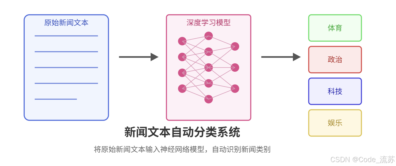
大家好，欢迎来到Python星球的第63天！🪐

在经过前62天的学习旅程，我们已经掌握了从Python基础到机器学习、深度学习的各种知识。今天，我们将把所学的知识综合应用到一个实际的文本分类项目中，实现新闻类别的自动分类系统。这个项目将综合运用文本处理、深度学习和Web开发技术，帮助我们巩固所学知识并拓展实战经验。

一、项目需求分析

1. 项目背景与目标

随着互联网信息爆炸式增长，自动文本分类技术在信息过滤、内容推荐等领域发挥着越来越重要的作用。我们的项目目标是构建一个能够自动将新闻文章分类到预定义类别（如体育、政治、科技、娱乐等）的系统。

在这里插入图片描述

2. 功能需求

能够接收新闻文本内容作为输入
对输入文本进行预处理
使用训练好的深度学习模型预测新闻类别
返回预测结果及置信度
提供REST API接口供其他系统调用

3. 技术方案概述

在这里插入图片描述

二、数据清洗与文本预处理

1. 数据集介绍

对于新闻分类项目，我们将使用THUCNews数据集，这是一个中文新闻数据集，包含财经、体育、娱乐等多个类别的新闻文本。当然，你也可以选择其他类似的数据集，如BBC News或20 Newsgroups。

# 数据集加载示例
import pandas as pd
import os# 定义数据路径
data_path = "./thucnews/"
categories = ['体育', '财经', '科技', '娱乐', '时政', '教育', '社会']# 读取数据
data = []
labels = []for category_id, category in enumerate(categories):category_path = os.path.join(data_path, category)files = os.listdir(category_path)for file in files:with open(os.path.join(category_path, file), 'r', encoding='utf-8') as f:content = f.read()data.append(content)labels.append(category_id)# 创建DataFrame
news_df = pd.DataFrame({'content': data,'category_id': labels,'category': [categories[i] for i in labels]
})print(f"数据集大小: {len(news_df)}")
print(news_df.category.value_counts())

2. 数据清洗步骤

文本数据通常需要经过一系列清洗和预处理步骤，以提高模型的训练效果：

在这里插入图片描述

下面我们来实现文本预处理的具体代码：

import re
import jieba
import numpy as np
from sklearn.model_selection import train_test_split# 1. 去除HTML标签
def remove_html_tags(text):"""去除文本中的HTML标签"""clean = re.compile('<.*?>')return re.sub(clean, '', text)# 2. 去除特殊字符
def remove_special_chars(text):"""去除特殊字符，只保留中文、英文、数字和基本标点"""return re.sub(r'[^\u4e00-\u9fa5a-zA-Z0-9，。！？、；：""''（）【】《》]', ' ', text)# 3. 中文分词
def chinese_word_cut(text):"""使用jieba进行中文分词"""return ' '.join(jieba.cut(text))# 4. 去除停用词
def remove_stopwords(text, stopwords_set):"""去除停用词"""words = text.split()filtered_words = [word for word in words if word not in stopwords_set]return ' '.join(filtered_words)# 加载停用词表
def load_stopwords(file_path='./stopwords.txt'):"""加载停用词表"""with open(file_path, 'r', encoding='utf-8') as f:stopwords = set([line.strip() for line in f.readlines()])return stopwords# 综合预处理函数
def preprocess_text(df, text_column='content', stopwords_path='./stopwords.txt'):"""对DataFrame中的文本列进行预处理"""# 加载停用词try:stopwords = load_stopwords(stopwords_path)except:print("停用词文件不存在，将不进行停用词过滤")stopwords = set()# 应用预处理函数df['clean_text'] = df[text_column].apply(remove_html_tags)df['clean_text'] = df['clean_text'].apply(remove_special_chars)df['clean_text'] = df['clean_text'].apply(chinese_word_cut)if stopwords:df['clean_text'] = df['clean_text'].apply(lambda x: remove_stopwords(x, stopwords))return df# 数据集划分
def split_dataset(df, test_size=0.2, val_size=0.1, random_state=42):"""将数据集划分为训练集、验证集和测试集"""# 先分离出测试集train_val, test = train_test_split(df, test_size=test_size, random_state=random_state, stratify=df['category_id'])# 从剩余数据中分离出验证集val_ratio = val_size / (1 - test_size)train, val = train_test_split(train_val, test_size=val_ratio, random_state=random_state, stratify=train_val['category_id'])print(f"训练集大小: {len(train)}")print(f"验证集大小: {len(val)}")print(f"测试集大小: {len(test)}")return train, val, test# 应用到我们的数据集
news_df_clean = preprocess_text(news_df)
train_df, val_df, test_df = split_dataset(news_df_clean)

3. 文本向量化

在深度学习模型中，我们需要将文本转换为数值向量形式。主要有以下几种方法：

One-hot编码：最简单的表示形式，但维度高、稀疏
词袋模型(Bag of Words)：统计词频，忽略词序
TF-IDF：考虑词在文档和语料库中的重要性
词嵌入(Word Embedding)：如Word2Vec、GloVe，能捕捉语义关系
预训练语言模型：如BERT的embedding层输出

对于我们的项目，将使用词嵌入和序列填充的方式：

from tensorflow.keras.preprocessing.text import Tokenizer
from tensorflow.keras.preprocessing.sequence import pad_sequences# 1. 创建分词器
max_words = 50000  # 词汇表大小
tokenizer = Tokenizer(num_words=max_words, oov_token='<UNK>')
tokenizer.fit_on_texts(train_df['clean_text'])# 词汇表大小
vocab_size = min(max_words, len(tokenizer.word_index) + 1)
print(f"词汇表大小: {vocab_size}")# 2. 转换文本为序列
train_sequences = tokenizer.texts_to_sequences(train_df['clean_text'])
val_sequences = tokenizer.texts_to_sequences(val_df['clean_text'])
test_sequences = tokenizer.texts_to_sequences(test_df['clean_text'])# 3. 序列填充
max_seq_length = 200  # 最大序列长度
train_padded = pad_sequences(train_sequences, maxlen=max_seq_length, padding='post', truncating='post')
val_padded = pad_sequences(val_sequences, maxlen=max_seq_length, padding='post', truncating='post')
test_padded = pad_sequences(test_sequences, maxlen=max_seq_length, padding='post', truncating='post')# 4. 准备标签
from tensorflow.keras.utils import to_categoricaltrain_labels = to_categorical(train_df['category_id'])
val_labels = to_categorical(val_df['category_id']) 
test_labels = to_categorical(test_df['category_id'])print(f"特征形状: {train_padded.shape}")
print(f"标签形状: {train_labels.shape}")

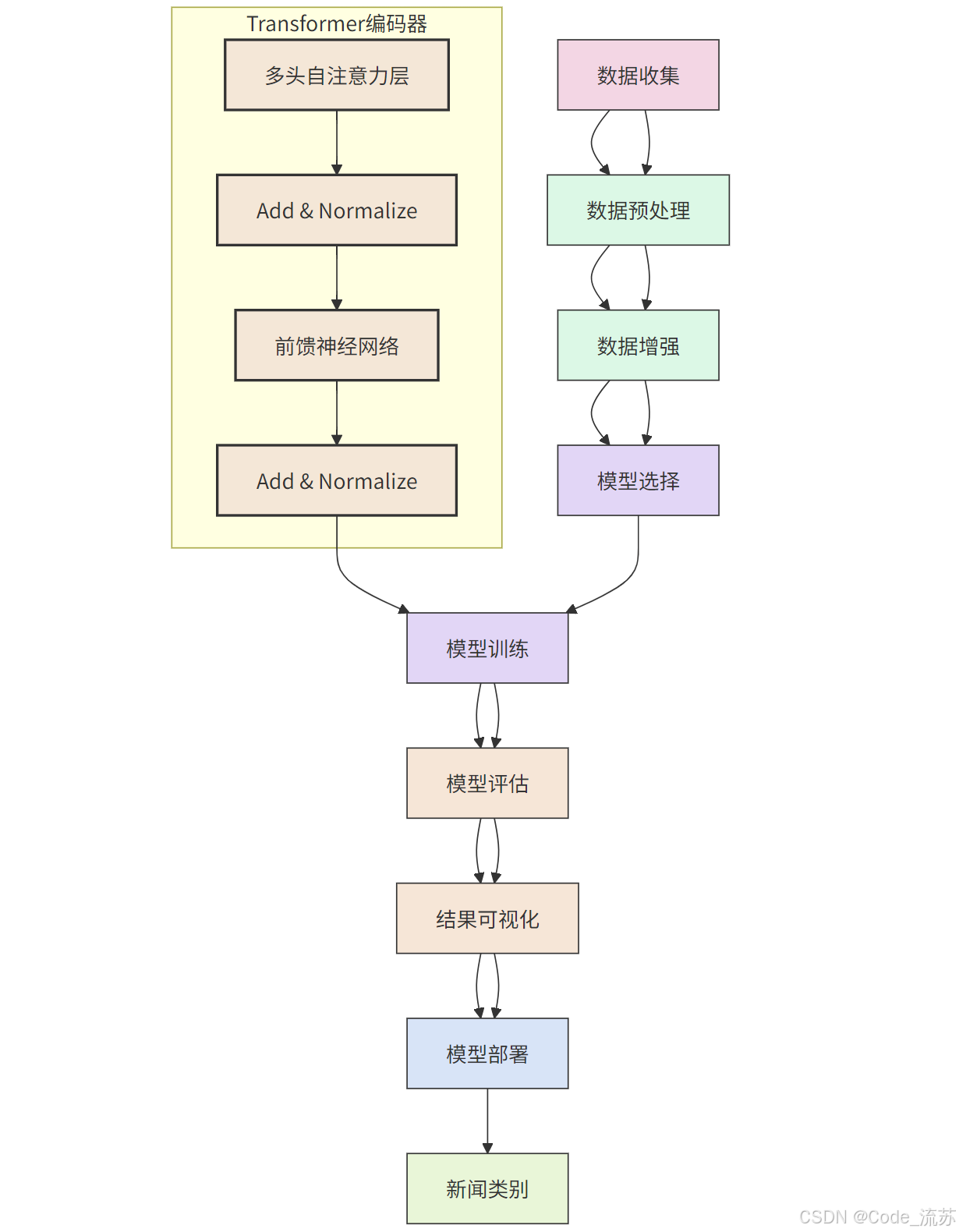
三、模型选择与训练

对于文本分类任务，我们将尝试三种不同的深度学习模型架构：RNN、LSTM和Transformer，然后比较它们的性能。

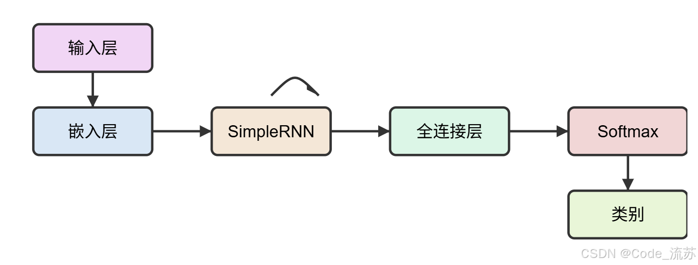
1. RNN模型

循环神经网络(RNN)是处理序列数据的基础模型，但存在长序列梯度消失问题。

在这里插入图片描述

from tensorflow.keras.models import Sequential
from tensorflow.keras.layers import Dense, Embedding, SimpleRNN, Dropout# RNN模型构建
def build_rnn_model(vocab_size, embedding_dim=100, max_length=200, num_classes=7):model = Sequential([# 嵌入层将词索引转换为密集向量Embedding(vocab_size, embedding_dim, input_length=max_length),# SimpleRNN层处理序列信息SimpleRNN(128, dropout=0.2, recurrent_dropout=0.2),# Dense层进行分类Dense(64, activation='relu'),Dropout(0.5),Dense(num_classes, activation='softmax')])# 编译模型model.compile(loss='categorical_crossentropy',optimizer='adam',metrics=['accuracy'])return model# 构建模型
embedding_dim = 100  # 词嵌入维度
rnn_model = build_rnn_model(vocab_size, embedding_dim, max_seq_length, len(categories))
rnn_model.summary()# 训练模型
rnn_history = rnn_model.fit(train_padded, train_labels,epochs=10,validation_data=(val_padded, val_labels),batch_size=64
)

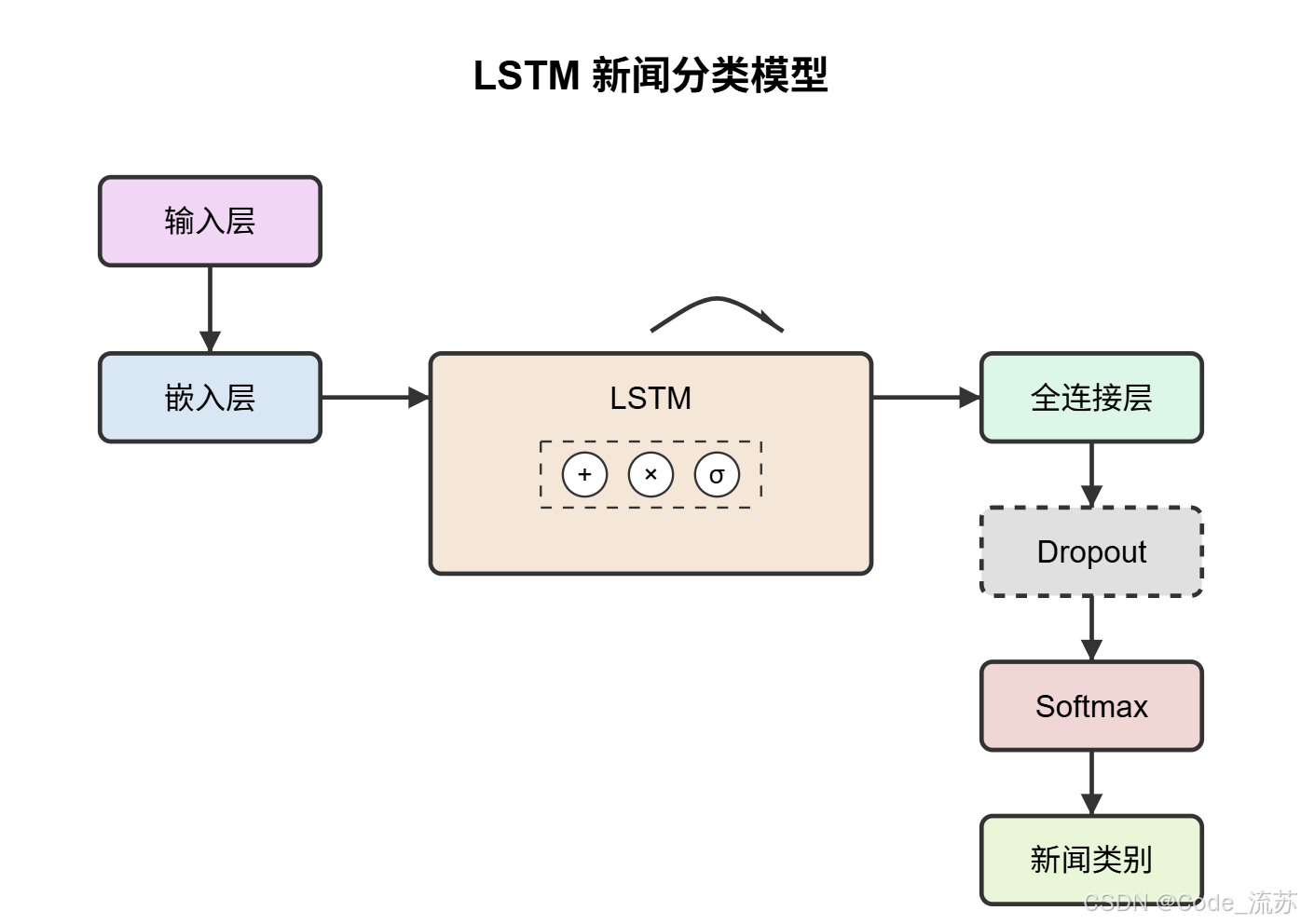
2. LSTM模型

长短期记忆网络(LSTM)是RNN的一种改进，能更好地处理长序列依赖问题。

在这里插入图片描述

from tensorflow.keras.layers import LSTM, Bidirectional# LSTM模型构建
def build_lstm_model(vocab_size, embedding_dim=100, max_length=200, num_classes=7):model = Sequential([# 嵌入层Embedding(vocab_size, embedding_dim, input_length=max_length),# 双向LSTM层可以捕捉前后文信息Bidirectional(LSTM(128, dropout=0.2, recurrent_dropout=0.2, return_sequences=True)),Bidirectional(LSTM(64, dropout=0.2, recurrent_dropout=0.2)),# Dense层进行分类Dense(64, activation='relu'),Dropout(0.5),Dense(num_classes, activation='softmax')])# 编译模型model.compile(loss='categorical_crossentropy',optimizer='adam',metrics=['accuracy'])return model# 构建模型
lstm_model = build_lstm_model(vocab_size, embedding_dim, max_seq_length, len(categories))
lstm_model.summary()# 训练模型
lstm_history = lstm_model.fit(train_padded, train_labels,epochs=10,validation_data=(val_padded, val_labels),batch_size=32  # LSTM更复杂，可以适当减小batch_size
)

3. Transformer模型

Transformer模型通过自注意力机制能够并行处理序列数据，是最新的NLP架构。

在这里插入图片描述

import tensorflow as tf
from tensorflow.keras.layers import Input, GlobalAveragePooling1D, LayerNormalization, MultiHeadAttention, Dense, Dropout, Embedding# Transformer模型构建
def build_transformer_model(vocab_size, embedding_dim=100, max_length=200, num_classes=7):# 输入层inputs = Input(shape=(max_length,))# 嵌入层embedding_layer = Embedding(vocab_size, embedding_dim)(inputs)# 位置编码（简化版，实际应用中可以使用三角函数实现）positions = tf.range(start=0, limit=max_length, delta=1)positions = Embedding(max_length, embedding_dim)(positions)x = embedding_layer + positions# Transformer编码器块num_heads = 8  # 注意力头数ff_dim = 256   # 前馈网络维度# 多头自注意力attention_output = MultiHeadAttention(num_heads=num_heads, key_dim=embedding_dim // num_heads)(x, x)attention_output = Dropout(0.1)(attention_output)x = LayerNormalization(epsilon=1e-6)(x + attention_output)# 前馈神经网络ffn_output = Dense(ff_dim, activation="relu")(x)ffn_output = Dense(embedding_dim)(ffn_output)ffn_output = Dropout(0.1)(ffn_output)x = LayerNormalization(epsilon=1e-6)(x + ffn_output)# 全局池化x = GlobalAveragePooling1D()(x)# 输出层x = Dense(64, activation="relu")(x)x = Dropout(0.5)(x)outputs = Dense(num_classes, activation="softmax")(x)# 构建模型model = tf.keras.Model(inputs=inputs, outputs=outputs)# 编译模型model.compile(optimizer="adam",loss="categorical_crossentropy",metrics=["accuracy"])return model# 构建模型
transformer_model = build_transformer_model(vocab_size, embedding_dim, max_seq_length, len(categories))
transformer_model.summary()# 训练模型
transformer_history = transformer_model.fit(train_padded, train_labels,epochs=10,validation_data=(val_padded, val_labels),batch_size=16  # Transformer更复杂，进一步减小batch_size
)

4. 模型比较与选择

我们需要对比三种模型在测试集上的表现，选择最佳模型：

import matplotlib.pyplot as plt
from sklearn.metrics import classification_report, confusion_matrix
import seaborn as sns# 绘制训练历史
def plot_history(histories, names):plt.figure(figsize=(12, 5))# 绘制准确率plt.subplot(1, 2, 1)for i, history in enumerate(histories):plt.plot(history.history['accuracy'], label=f'{names[i]} Train')plt.plot(history.history['val_accuracy'], label=f'{names[i]} Val')plt.title('模型准确率')plt.ylabel('准确率')plt.xlabel('轮次')plt.legend()# 绘制损失plt.subplot(1, 2, 2)for i, history in enumerate(histories):plt.plot(history.history['loss'], label=f'{names[i]} Train')plt.plot(history.history['val_loss'], label=f'{names[i]} Val')plt.title('模型损失')plt.ylabel('损失')plt.xlabel('轮次')plt.legend()plt.tight_layout()plt.show()# 评估模型
def evaluate_model(model, test_data, test_labels, name, tokenizer=None, categories=None):# 预测y_pred_probs = model.predict(test_data)y_pred = np.argmax(y_pred_probs, axis=1)y_true = np.argmax(test_labels, axis=1)# 打印分类报告print(f"===== {name} 模型评估 =====")print(classification_report(y_true, y_pred, target_names=categories))# 绘制混淆矩阵plt.figure(figsize=(10, 8))cm = confusion_matrix(y_true, y_pred)sns.heatmap(cm, annot=True, fmt='d', cmap='Blues', xticklabels=categories, yticklabels=categories)plt.title(f'{name} 混淆矩阵')plt.ylabel('真实类别')plt.xlabel('预测类别')plt.tight_layout()plt.show()return y_pred_probs# 比较三个模型
histories = [rnn_history, lstm_history, transformer_history]
names = ['RNN', 'LSTM', 'Transformer']
plot_history(histories, names)# 评估各个模型
rnn_probs = evaluate_model(rnn_model, test_padded, test_labels, 'RNN', tokenizer, categories)
lstm_probs = evaluate_model(lstm_model, test_padded, test_labels, 'LSTM', tokenizer, categories)
transformer_probs = evaluate_model(transformer_model, test_padded, test_labels, 'Transformer', tokenizer, categories)# 假设LSTM模型表现最好，我们选择它作为最终模型
best_model = lstm_model
best_model.save('news_classifier_lstm.h5')

四、结果可视化与评估

1. 类别分布与预测置信度

可视化模型对各个类别的识别能力和置信度分布：

import matplotlib.pyplot as plt
import numpy as np
import seaborn as sns# 获取预测结果
y_pred_probs = best_model.predict(test_padded)
y_pred = np.argmax(y_pred_probs, axis=1)
y_true = np.argmax(test_labels, axis=1)# 1. 类别分布可视化
plt.figure(figsize=(12, 6))
plt.subplot(1, 2, 1)
sns.countplot(x=[categories[i] for i in y_true])
plt.title('真实类别分布')
plt.xticks(rotation=45)plt.subplot(1, 2, 2)
sns.countplot(x=[categories[i] for i in y_pred])
plt.title('预测类别分布')
plt.xticks(rotation=45)
plt.tight_layout()
plt.show()# 2. 预测置信度分布
plt.figure(figsize=(10, 6))
# 获取每个预测的最大置信度
confidences = np.max(y_pred_probs, axis=1)
# 按类别分组置信度
confidence_by_category = {}
for i, category_id in enumerate(y_pred):category = categories[category_id]if category not in confidence_by_category:confidence_by_category[category] = []confidence_by_category[category].append(confidences[i])# 使用箱形图显示每个类别的置信度分布
data = []
labels = []
for category, confs in confidence_by_category.items():data.extend(confs)labels.extend([category] * len(confs))sns.boxplot(x=labels, y=data)
plt.title('各类别预测置信度分布')
plt.ylabel('置信度')
plt.xlabel('类别')
plt.xticks(rotation=45)
plt.tight_layout()
plt.show()

2. 错误分析

分析模型错误预测的案例，了解模型的局限性：

# 错误预测案例分析
def analyze_errors(model, test_data, test_texts, y_true, categories, n_examples=5):"""分析错误预测的案例"""y_pred_probs = model.predict(test_data)y_pred = np.argmax(y_pred_probs, axis=1)# 找出错误预测的索引error_indices = np.where(y_pred != y_true)[0]if len(error_indices) == 0:print("没有发现错误预测")return# 随机选择n个错误例子selected_indices = np.random.choice(error_indices, min(n_examples, len(error_indices)), replace=False)print("===== 错误预测案例分析 =====")for i, idx in enumerate(selected_indices):true_category = categories[y_true[idx]]pred_category = categories[y_pred[idx]]confidence = y_pred_probs[idx][y_pred[idx]] * 100print(f"案例 {i+1}:")print(f"文本: {test_texts[idx][:200]}...")  # 只显示前200个字符print(f"真实类别: {true_category}")print(f"预测类别: {pred_category}")print(f"预测置信度: {confidence:.2f}%")print(f"可能原因: {'过度依赖特定关键词' if confidence > 90 else '内容主题混合或边界模糊'}")print('-' * 50)# 获取测试集文本
test_texts = test_df['clean_text'].tolist()
analyze_errors(best_model, test_padded, test_texts, y_true, categories)

3. 词云可视化

通过词云了解每个类别的特征词：

from wordcloud import WordCloud
import matplotlib.pyplot as plt
import jieba
from collections import Counter# 为每个类别生成词云
def generate_wordclouds(df, text_column, category_column, categories):"""为每个类别生成词云"""plt.figure(figsize=(15, 10))for i, category in enumerate(categories):# 获取该类别的所有文本category_texts = df[df[category_column] == category][text_column].tolist()if not category_texts:continue# 将所有文本合并combined_text = ' '.join(category_texts)# 分词并统计词频words = jieba.cut(combined_text)word_counts = Counter(words)# 过滤掉停用词和单个字符word_counts = {word: count for word, count in word_counts.items() if len(word) > 1 and word.strip()}# 生成词云wordcloud = WordCloud(font_path='simhei.ttf',  # 指定中文字体width=400, height=300, background_color='white').generate_from_frequencies(word_counts)# 绘制词云plt.subplot(2, 4, i+1)plt.imshow(wordcloud, interpolation='bilinear')plt.title(category)plt.axis('off')plt.tight_layout()plt.show()# 生成每个类别的词云
generate_wordclouds(train_df, 'clean_text', 'category', categories)

五、模型部署与API构建

1. 构建RESTful API

使用Flask框架构建简单的REST API：

from flask import Flask, request, jsonify
import tensorflow as tf
import numpy as np
import pickle
import re
import jiebaapp = Flask(__name__)# 加载必要的组件
def load_model_components():"""加载模型和预处理组件"""# 加载模型model = tf.keras.models.load_model('news_classifier_lstm.h5')# 加载分词器with open('tokenizer.pickle', 'rb') as handle:tokenizer = pickle.load(handle)# 加载类别标签categories = ['体育', '财经', '科技', '娱乐', '时政', '教育', '社会']# 加载停用词try:with open('stopwords.txt', 'r', encoding='utf-8') as f:stopwords = set([line.strip() for line in f.readlines()])except:stopwords = set()return model, tokenizer, categories, stopwords# 预处理函数
def preprocess_text(text, stopwords):"""文本预处理"""# 去除HTML标签clean = re.compile('<.*?>')text = re.sub(clean, '', text)# 去除特殊字符text = re.sub(r'[^\u4e00-\u9fa5a-zA-Z0-9，。！？、；：""''（）【】《》]', ' ', text)# 分词words = jieba.cut(text)# 去除停用词if stopwords:words = [word for word in words if word not in stopwords]return ' '.join(words)# 模型预测
def predict_category(text, model, tokenizer, categories, max_length=200):"""预测文本类别"""# 预处理文本processed_text = preprocess_text(text, stopwords)# 文本转序列sequence = tokenizer.texts_to_sequences([processed_text])# 序列填充padded = tf.keras.preprocessing.sequence.pad_sequences(sequence, maxlen=max_length, padding='post', truncating='post')# 预测prediction = model.predict(padded)[0]# 获取结果category_id = np.argmax(prediction)category = categories[category_id]confidence = float(prediction[category_id])# 获取各类别置信度category_confidences = {cat: float(prediction[i]) for i, cat in enumerate(categories)}return {'category': category,'confidence': confidence,'category_confidences': category_confidences}# 全局加载模型和预处理组件
print("加载模型和预处理组件...")
model, tokenizer, categories, stopwords = load_model_components()
print("模型加载完成！")# API路由
@app.route('/predict', methods=['POST'])
def predict():"""预测API路由"""# 获取请求数据data = request.json# 检查请求是否包含文本if 'text' not in data:return jsonify({'error': '请求中缺少文本字段'}), 400# 执行预测try:result = predict_category(data['text'], model, tokenizer, categories)return jsonify(result)except Exception as e:return jsonify({'error': str(e)}), 500# 健康检查路由
@app.route('/health', methods=['GET'])
def health():"""健康检查路由"""return jsonify({'status': 'ok'})if __name__ == '__main__':app.run(debug=True, host='0.0.0.0', port=5000)

2. 保存和加载组件

为了部署API，我们需要保存模型、分词器和其他必要组件：

# 保存分词器
import pickle
with open('tokenizer.pickle', 'wb') as handle:pickle.dump(tokenizer, handle, protocol=pickle.HIGHEST_PROTOCOL)# 保存模型
best_model.save('news_classifier_lstm.h5')# 保存停用词（如果使用）
with open('stopwords.txt', 'w', encoding='utf-8') as f:for word in stopwords:f.write(f"{word}\n")print("模型和预处理组件已保存！")

3. 部署建议

推荐使用Docker容器化部署我们的API服务，下面是一个简单的Dockerfile示例：

# Dockerfile
FROM python:3.8-slimWORKDIR /app# 复制必要文件
COPY requirements.txt .
COPY app.py .
COPY news_classifier_lstm.h5 .
COPY tokenizer.pickle .
COPY stopwords.txt .# 安装依赖
RUN pip install --no-cache-dir -r requirements.txt# 暴露端口
EXPOSE 5000# 启动应用
CMD ["python", "app.py"]

requirements.txt文件内容：

flask==2.0.1
tensorflow==2.6.0
numpy==1.19.5
jieba==0.42.1

4. 使用示例

下面是一个使用curl调用API的示例：

curl -X POST http://localhost:5000/predict \-H "Content-Type: application/json" \-d '{"text": "2025年第一季度，中国经济增长6.3%，这一数据超出市场预期。专家认为，消费需求回暖和出口增长是主要推动因素。"}'

返回结果示例：

{"category": "财经","confidence": 0.9782,"category_confidences": {"体育": 0.0002,"财经": 0.9782,"科技": 0.0132,"娱乐": 0.0003,"时政": 0.0065,"教育": 0.0008,"社会": 0.0008}
}