当前位置：首页 > news >正文

项目实战-基于信号处理与SVM机器学习的声音情感识别系统

news 2025/5/6 6:43:40

一.背景描述

二.理论部分

三.程序设计

编程思路

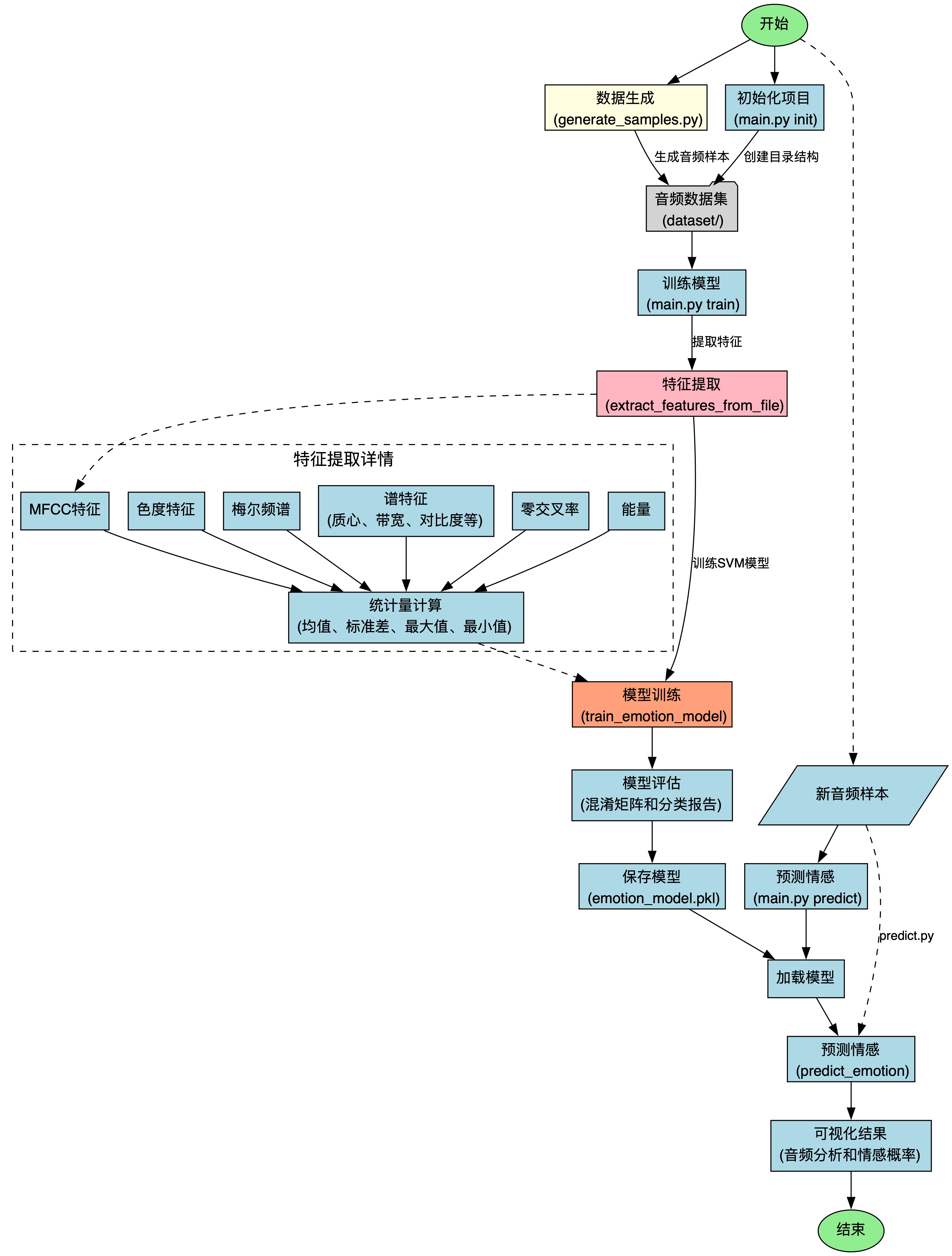
流程图

1.信号部分创建数据 generate_samples.py

头文件

生成函数 generate_emotion_sample

传入参数

存储路径

生成参数

创建基础正弦波信号

调制基础正弦波

对于愤怒可以增加噪声

归一化信号

存储

主函数 main

2.交叉部分特征提取 audio_emotion.py

头文件

提取单个文件的特征 extract_features_from_file

传入参数

提取特征向量

计算统计值并返回矩阵

提取各情感的特征 extract_features_from_directory

传入参数

初始化

提取文件 & 识别特征

训练情感识别模型 train_emotion_model

传入参数

划分训练集和测试集

训练SVM模型

评估测试集

计算混淆矩阵

保存模型

加载模型

预测单个音频的情感

混淆矩阵可视化

音频特征可视化

传入参数

处理音频

特征提取

可视化并保存

3.机器学习部分 train_model.py

为何要独立出一个训练脚本

头文件

主函数 main

4.封装部分 main.py

创建项目目录

提取特征并训练模型

预测单个文件情感

显示

主逻辑

5.预测部分 predict.py

头文件

可视化音频特征

主逻辑

应用

四.运行展示

初始化目录

生成样本

训练模型

查看结果并分析

应用模型

查看分析图

一.背景描述

智能识别不同情景下的声音信号体现的情感，比如客户接电话时的语音情感，还可以用于智能手表、人工智能助手（比如豆包的聊天过程中的人类情感反馈，提高豆包“情商”）等等

二.理论部分

1.首先分析了不同情感声音信号的特征，用于下面的构造信号

2.构造不同情感的声音信号（通过将时间序列代入基准正弦信号，接着进行加、乘操作进行调制）用于训练SVM模型

3.对信号进行时频域变换，比如傅立叶变换

chroma = librosa.feature.chroma_stft(y=y, sr=sr)

4.进行特征提取，捕捉谱质心、谱带宽、谱对比度等等

5.进行特征的统计，计算了四种统计量：均值、标准差、最小值、最大值

6.通过均方根计算能量，这是情感表达的重要指标

7.特征空间降维，通过统计的方式进行了隐式降维

三.程序设计

编程思路

整体框架是：

1.信号生成 generate_samples.py

2.特征提取 audio_emotion.py

3.训练模型 train_model.py

4.封装模块 main.py

5.应用模型 predict.py

流程图

1.信号部分创建数据 generate_samples.py

头文件

import os
import numpy as np
import librosa
import soundfile as sf
from scipy.io import wavfile

生成函数 generate_emotion_sample

传入参数

emotion 情感

freq_range 生成音频信号的频率范围

duration_range 生成信号的持续时间范围

num_samples 生成的音频样本数量

存储路径

    emotion_dir = os.path.join("dataset", emotion)os.makedirs(emotion_dir, exist_ok=True)

dataset 是数据集的根目录，在根目录下创建名为传入参数emotion的子目录

第二句的作用是保证文件夹存在

生成参数

首先我们得明确各情感声音特色

"happy"：高频、短持续时间，模拟快乐情感。
"sad"：低频、长持续时间，模拟悲伤情感。
"angry"：中高频、短脉冲，模拟愤怒情感。
"neutral"：中等频率和持续时间，模拟中性情感。

那么我们只需要判断，然后分支为各情感创建独特的参数就好

以“happy”为例

首先我们要从指定的频率中随机选择频率值，对应下面的np.random.uniform(freq_range[0], freq_range[1])语句，里面的freq_range[ 0 ] 和 freq_range[1] 分别代表频率范围的上下限，我们会在主函数中提前定义

（注意：我们这里得用numpy的random，而不是python自带的random函数，因为np的支持数组高效操作）

然后我们还需要持续时间，和频率同理也是np.random.uniform

接着我们设置了音频信号的振幅频率（音量），快乐的声音为0.6中等偏高来模拟

最后我们设置振幅调制的频率，快乐的是8.0：快速的变化，模拟快乐的活泼

其他的感情和快乐同理

    for i in range(num_samples):if emotion == "happy":# 高频和短持续时间freq = np.random.uniform(freq_range[0], freq_range[1])duration = np.random.uniform(duration_range[0], duration_range[1])amplitude = 0.6modulation_freq = 8.0elif emotion == "sad":# 低频和长持续时间freq = np.random.uniform(freq_range[0]/2, freq_range[1]/2)duration = np.random.uniform(duration_range[0]*1.5, duration_range[1]*1.5)amplitude = 0.4modulation_freq = 2.0elif emotion == "angry":# 中高频和短脉冲freq = np.random.uniform(freq_range[0]*1.2, freq_range[1]*1.2)duration = np.random.uniform(duration_range[0], duration_range[1])amplitude = 0.8modulation_freq = 12.0else:  # neutral# 中等频率和持续时间freq = np.random.uniform(freq_range[0]*0.8, freq_range[1]*0.8)duration = np.random.uniform(duration_range[0]*1.2, duration_range[1]*1.2)amplitude = 0.5modulation_freq = 4.0

创建基础正弦波信号

        sample_rate = 22050t = np.linspace(0, duration, int(sample_rate * duration), endpoint=False)signal = amplitude * np.sin(2 * np.pi * freq * t)

首先我们设置了音频信号的采样频率，单位是“样本/秒”

然后我们用 numpy 的 linspace 创建了一个时间序列，用于表示信号的时间轴，第一个参数0表示时间序列起点，duration是时间序列的终点（也就是我们在上面生成的持续时间），第三个参数是时间序列的点数（计算方式：采样率乘以持续时间），endpoint保证时间序列不包含终点

然后我们生成一个正弦波信号，amplitude表示正弦波的振幅（音量），freq时频率（音调），t是上面生成的时间序列，通过 2 * np.pi * freq * t 将频率转为角频率，计算正弦波的相位

调制基础正弦波

我们还需要根据我们的情感对基础波进行处理

        modulation = 1.0 + 0.3 * np.sin(2 * np.pi * modulation_freq * t)signal = signal * modulation

modulation是生成的调制信号，用于改变原始信号的振幅，其中 1.0 是基础振幅（乘法的初元）， 0.3表示调制强度（影响程度）

第二句代码也就是将调制信号作用在原正弦波signal上

对于愤怒可以增加噪声

对于“angry”：加上信号

        if emotion == "angry":noise = np.random.normal(0, 0.1, signal.shape)signal = signal + noise

归一化信号

进行归一化：除以max乘以1

限制信号在 [ -1,1 ] 中，确保生成的音频信号符合音频文件格式的要求，防止信号溢出

        signal = signal / np.max(np.abs(signal))

存储

        file_path = os.path.join(emotion_dir, f"{emotion}_sample_{i+1}.wav")sf.write(file_path, signal, sample_rate)print(f"生成样本: {file_path}")

emotion_dir 在函数刚进来一开始就定义了

然后我加了一句print方便调试看报错

主函数 main

def main():freq_range = (220, 880)duration_range = (2.0, 4.0)emotions = ["happy", "sad", "angry", "neutral"]for emotion in emotions:generate_emotion_sample(emotion, freq_range, duration_range, num_samples=50)print("所有测试样本生成完成！")if __name__ == "__main__":main()

freq_range 是频率范围

duration_range 是持续时间

num是生成数据集的个数，我先设置为50（多多益善）

然后用 for 遍历感情

2.交叉部分特征提取 audio_emotion.py

头文件

import os
import numpy as np
import librosa
import librosa.display 
import matplotlib.pyplot as plt
from sklearn.model_selection import train_test_split
from sklearn.svm import SVC
from sklearn.metrics import classification_report, confusion_matrix
import joblib
import glob

提取单个文件的特征 extract_features_from_file

传入参数

file_path 文件的路径

win 计算特征的时间窗口长度

step 步长

提取特征向量

先读取音频文件

        y, sr = librosa.load(file_path, sr=None)

读取MFCC特征

        mfccs = librosa.feature.mfcc(y=y, sr=sr, n_mfcc=13)

提取色度特征

        chroma = librosa.feature.chroma_stft(y=y, sr=sr)

提取梅尔频谱

        mel = librosa.feature.melspectrogram(y=y, sr=sr)

提取谱质心

        spectral_centroid = librosa.feature.spectral_centroid(y=y, sr=sr)

提取谱带宽

        spectral_bandwidth = librosa.feature.spectral_bandwidth(y=y, sr=sr)

提取谱对比度

        spectral_contrast = librosa.feature.spectral_contrast(y=y, sr=sr)

提取谱平坦度

        spectral_flatness = librosa.feature.spectral_flatness(y=y)

提取零交叉率

        zcr = librosa.feature.zero_crossing_rate(y)

提取能量

        energy = np.mean(librosa.feature.rms(y=y))

计算统计值并返回矩阵

        features.append(energy)feature_names = []for name in ['mfccs', 'chroma', 'mel', 'spectral_centroid', 'spectral_bandwidth', 'spectral_contrast', 'spectral_flatness', 'zcr']:for stat in ['mean', 'std', 'min', 'max']:feature_names.append(f"{name}_{stat}")feature_names.append('energy')return np.array(features), feature_names

提取各情感的特征 extract_features_from_directory

传入参数

directory 数据集根目录

emotions 情感类别

初始化

    features = []labels = []feature_names = None

其中

feature 特征向量

labels 情感标签

feature_names 特征的名称列表

提取文件 & 识别特征

首先我加了一句 print 方便调试

    print(f"开始从以下类别提取特征: {emotions}")for emotion in emotions:emotion_dir = os.path.join(directory, emotion)if not os.path.isdir(emotion_dir):continuefor file_name in glob.glob(os.path.join(emotion_dir, "*.wav")):print(f"处理文件: {file_name}")feature_vector, names = extract_features_from_file(file_name)if feature_vector is not None:features.append(feature_vector)labels.append(emotion)if feature_names is None:feature_names = names

然后我们开始

遍历情感类别 for emotion in emotions（如果子目录不存在那就continue跳过）

遍历音频文件 for file_name in glob.glob(os.path.join(emotion_dir, "*.wav"))

提取音频特征对于提取到的单个文件开始调用extract_features_from_file

存储特征和标签 append

最后我们返回

    return np.array(features), np.array(labels), feature_names

后面的就是机器学习部分

训练情感识别模型 train_emotion_model

传入参数

feature 特征矩阵，每一行都是一个音频的特征向量，包含提取到的各种统计特征

labels 标签数组

test_size 测试集的比例，一般正常训练都是占比20%到30%，本次项目中设为0.2

划分训练集和测试集

    X_train, X_test, y_train, y_test = train_test_split(features, labels, test_size=test_size, random_state=42)

训练SVM模型

    model = SVC(kernel='rbf', probability=True)model.fit(X_train, y_train)

评估测试集

    y_pred = model.predict(X_test)report = classification_report(y_test, y_pred, output_dict=True)

计算混淆矩阵

    cm = confusion_matrix(y_test, y_pred)

model SVM模型

report 分类报告

cm 混淆矩阵

X_test 测试集的特征矩阵，来评估模型性能

y_test 测试集的真实标签，用于对比

y_pred 模型在测试集的预测标签，用于对比

    return model, report, cm, X_test, y_test, y_pred

保存模型

def save_model(model, output_path="emotion_model.pkl"):joblib.dump(model, output_path)print(f"模型已保存到 {output_path}")

加载模型

def load_model(model_path="emotion_model.pkl"):return joblib.load(model_path)

预测单个音频的情感

调用extract_features_from_file函数从指定file_path里面提取特征向量，然后特征预处理，将特征向量转换为模型可以接受的二维数组形状，接着调用model模型进行情感预测，返回每个情感类别的预测概率，便于分析模型的信心程度。这个函数在audio脚本中并没有被使用，而是在后面的main.py文件中被调用了

def predict_emotion(model, file_path):features, _ = extract_features_from_file(file_path)if features is not None:features = features.reshape(1, -1)prediction = model.predict(features)[0]probabilities = model.predict_proba(features)[0]return prediction, probabilitiesreturn None, None

混淆矩阵可视化

为了方便查看混淆矩阵，我用matplotlib来进行数据的可视化（由于我之前在数模比赛中做过斯皮尔曼相关矩阵的可视化，所以还是感觉轻车熟路的）

def visualize_confusion_matrix(cm, classes):plt.figure(figsize=(10, 8))plt.imshow(cm, interpolation='nearest', cmap=plt.cm.Blues)plt.title('混淆矩阵')plt.colorbar()tick_marks = np.arange(len(classes))plt.xticks(tick_marks, classes, rotation=45)plt.yticks(tick_marks, classes)thresh = cm.max() / 2.for i in range(cm.shape[0]):for j in range(cm.shape[1]):plt.text(j, i, format(cm[i, j], 'd'),horizontalalignment="center",color="white" if cm[i, j] > thresh else "black")plt.ylabel('真实标签')plt.xlabel('预测标签')plt.tight_layout()plt.savefig('confusion_matrix.png')plt.show()

效果展示

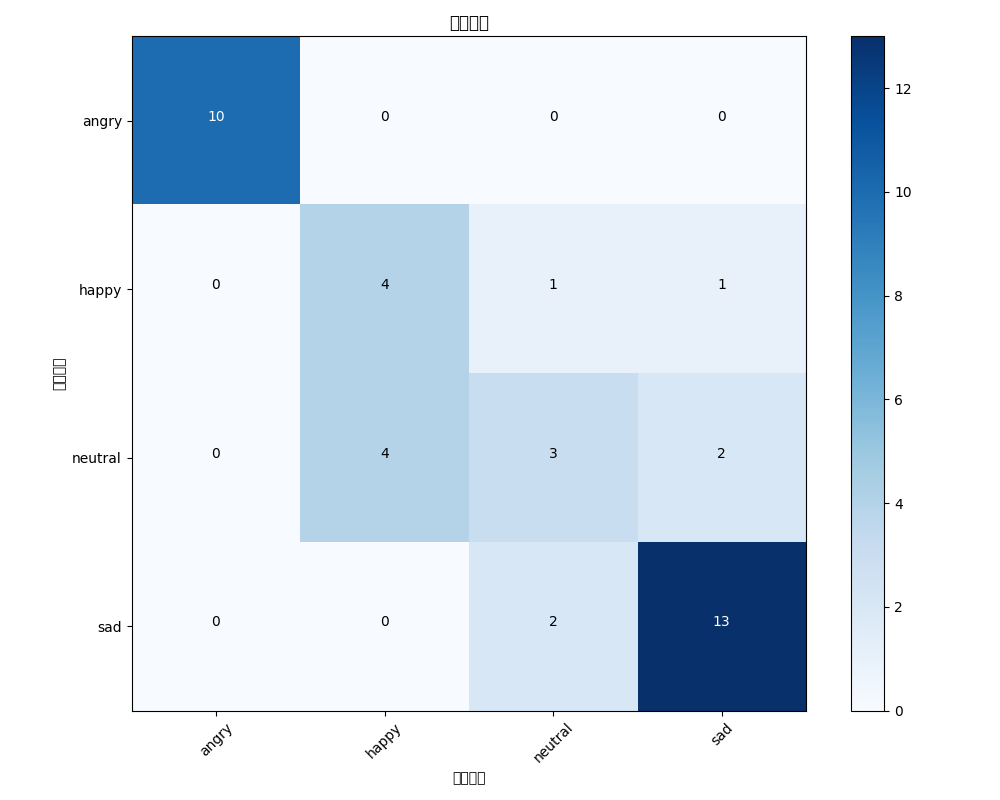
从图中可以直观的看到我们的模型准确率是不错的，具体的结论在后面分析

音频特征可视化

传入参数

audio_file 待分析的音频文件路径

处理音频

音频加载

y, sr = librosa.load(audio_file, sr=None)

音频持续时间计算

duration = librosa.get_duration(y=y, sr=sr)

特征提取

梅尔频谱

mel_spec = librosa.feature.melspectrogram(y=y, sr=sr)
mel_spec_db = librosa.power_to_db(mel_spec, ref=np.max)

MFCC（梅尔频谱倒谱系数）

mfccs = librosa.feature.mfcc(y=y, sr=sr, n_mfcc=13)

色度图

chroma = librosa.feature.chroma_stft(y=y, sr=sr)

可视化并保存

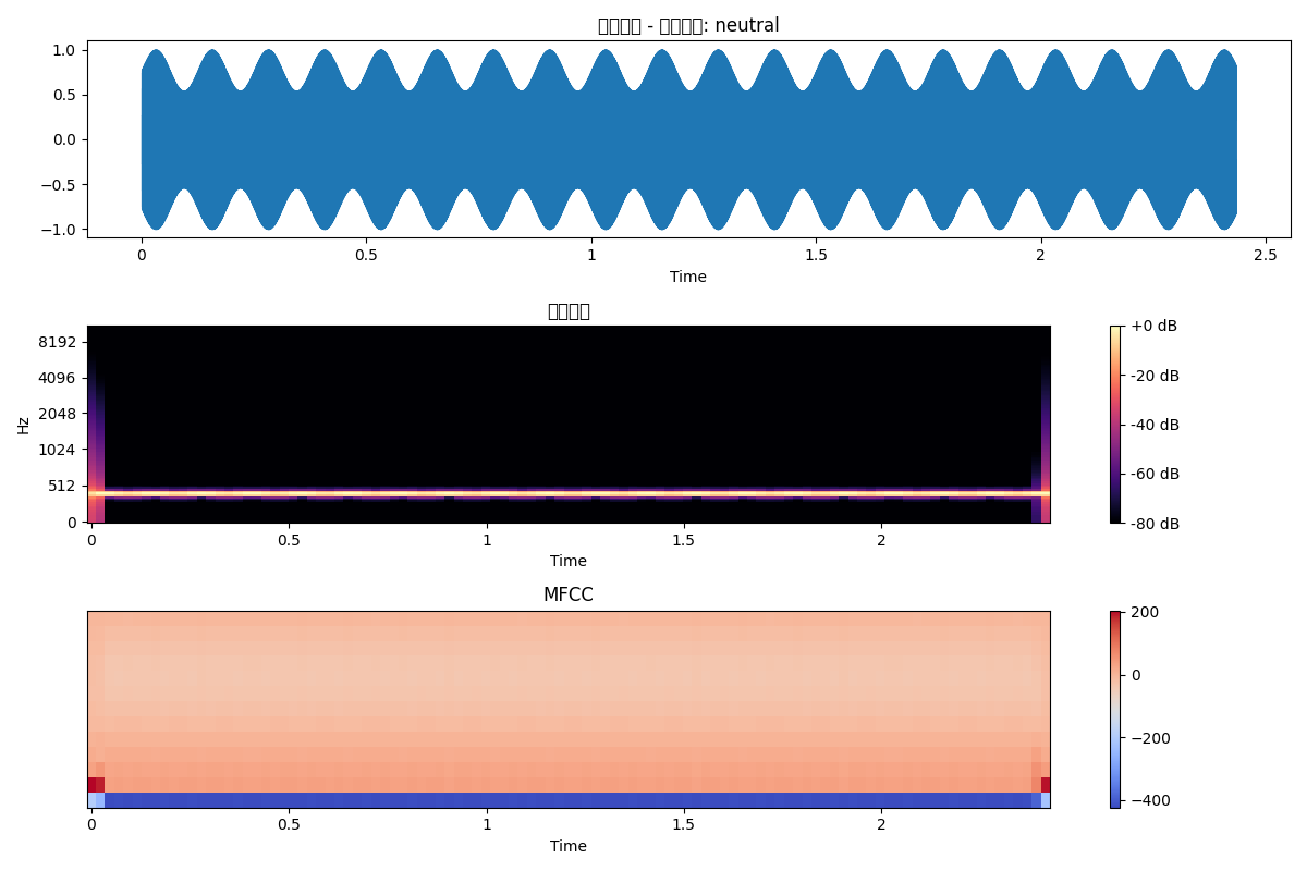
    plt.figure(figsize=(12, 10))# 波形plt.subplot(4, 1, 1)librosa.display.waveshow(y, sr=sr)plt.title('音频波形')# 梅尔频谱plt.subplot(4, 1, 2)librosa.display.specshow(mel_spec_db, sr=sr, x_axis='time', y_axis='mel')plt.colorbar(format='%+2.0f dB')plt.title('梅尔频谱')# MFCCplt.subplot(4, 1, 3)librosa.display.specshow(mfccs, sr=sr, x_axis='time')plt.colorbar()plt.title('MFCC')# 色度图plt.subplot(4, 1, 4)librosa.display.specshow(chroma, sr=sr, x_axis='time', y_axis='chroma')plt.colorbar()plt.title('色度图')plt.tight_layout()plt.savefig('audio_analysis.png')plt.show()

效果展现

将特征数据和原始数据返回，便于后面分析

return mel_spec, mfccs, chroma, sr, y

3.机器学习部分 train_model.py

为何要独立出一个训练脚本

可以看到我们之前在audio_emotion.py中包含了一系列功能，但是它只是一个功能库，并不会执行，只是定义了如何训练

那么我们就需要新写一个执行脚本来调用，他就是我们的train_model.py，这种模块化的设计方便我们更换不同的训练方法

头文件

import os
import numpy as np
import librosa
import matplotlib.pyplot as plt
from sklearn.model_selection import train_test_split
from sklearn.svm import SVC
from sklearn.metrics import classification_report, confusion_matrix
import joblib
import glob
import time
from audio_emotion import extract_features_from_file

设置输出日志

LOG_FILE = "training_log.txt"

写入输出日志

def log_message(message):print(message)with open(LOG_FILE, "a") as f:timestamp = time.strftime("%Y-%m-%d %H:%M:%S")f.write(f"[{timestamp}] {message}\n")

主函数 main

获取情感类别

    emotions = [d for d in os.listdir("dataset") if os.path.isdir(os.path.join("dataset", d))]

初始化特征和标签

    features = []labels = []feature_names = None

开始训练

    for emotion in emotions:emotion_dir = os.path.join("dataset", emotion)audio_files = glob.glob(os.path.join(emotion_dir, "*.wav"))if not audio_files:log_message(f"警告: {emotion} 类别中没有发现WAV文件。")continuelog_message(f"处理 {len(audio_files)} 个 {emotion} 类别的文件...")for audio_file in audio_files:log_message(f"提取特征: {audio_file}")feature_vector, names = extract_features_from_file(audio_file)  # 使用原始函数if feature_vector is not None:features.append(feature_vector)labels.append(emotion)if feature_names is None:feature_names = namesif not features:log_message("错误: 没有成功提取任何特征，请检查音频文件格式。")return# 转换为numpy数组features = np.array(features)labels = np.array(labels)log_message(f"成功提取 {len(features)} 个样本的特征，每个样本 {features.shape[1]} 个特征。")# 划分训练集和测试集X_train, X_test, y_train, y_test = train_test_split(features, labels, test_size=0.2, random_state=42)log_message(f"训练集: {X_train.shape[0]} 个样本，测试集: {X_test.shape[0]} 个样本。")# 训练SVM模型log_message("开始训练SVM模型...")model = SVC(kernel='rbf', probability=True)model.fit(X_train, y_train)log_message("SVM模型训练完成。")# 在测试集上评估y_pred = model.predict(X_test)# 计算分类报告report = classification_report(y_test, y_pred, output_dict=True)# 输出分类报告log_message("\n分类报告:")for emotion in sorted(report.keys()):if emotion != "accuracy" and emotion != "macro avg" and emotion != "weighted avg":precision = report[emotion]['precision']recall = report[emotion]['recall']f1 = report[emotion]['f1-score']support = report[emotion]['support']log_message(f"{emotion}:\t精确率: {precision:.2f}, 召回率: {recall:.2f}, F1: {f1:.2f}, 样本数: {support}")log_message(f"\n整体准确率: {report['accuracy']:.2f}")# 保存混淆矩阵log_message("生成混淆矩阵...")cm = confusion_matrix(y_test, y_pred)plt.figure(figsize=(10, 8))plt.imshow(cm, interpolation='nearest', cmap=plt.cm.Blues)plt.title('混淆矩阵')plt.colorbar()# 添加标签classes = sorted(np.unique(labels))tick_marks = np.arange(len(classes))plt.xticks(tick_marks, classes, rotation=45)plt.yticks(tick_marks, classes)# 在格子中添加数字thresh = cm.max() / 2.for i in range(cm.shape[0]):for j in range(cm.shape[1]):plt.text(j, i, format(cm[i, j], 'd'),horizontalalignment="center",color="white" if cm[i, j] > thresh else "black")plt.ylabel('真实标签')plt.xlabel('预测标签')plt.tight_layout()# 保存混淆矩阵图像plt.savefig('confusion_matrix.png')log_message("混淆矩阵已保存为 confusion_matrix.png")# 保存模型joblib.dump(model, 'emotion_model.pkl')log_message("模型已保存到 emotion_model.pkl")log_message("模型训练和评估完成！")

4.封装部分 main.py

最后我们还需要一个命令行界面用于调用模块、封装框架，他就是main文件

创建项目目录

def create_project_structure():print("开始创建项目目录结构...")os.makedirs("dataset", exist_ok=True)emotions = ["happy", "sad", "angry", "neutral"]for emotion in emotions:os.makedirs(os.path.join("dataset", emotion), exist_ok=True)print("项目目录结构已创建，请将音频文件放入相应的情感文件夹中：")print("  - dataset/happy/")print("  - dataset/sad/")print("  - dataset/angry/")print("  - dataset/neutral/")

提取特征并训练模型

def extract_and_train():if not os.path.exists("dataset"):print("数据集目录不存在，请先运行 'python main.py init'")returnprint("开始提取特征...")try:features, labels, feature_names = extract_features_from_directory("dataset")if len(features) == 0:print("未找到有效的特征数据，请确保数据集中包含.wav文件")returnprint(f"共提取了 {len(features)} 个样本的特征")# 训练模型print("开始训练模型...")model, report, cm, X_test, y_test, y_pred = train_emotion_model(features, labels)# 保存模型save_model(model)# 输出分类报告print("\n分类报告:")for emotion in report.keys():if emotion != "accuracy" and emotion != "macro avg" and emotion != "weighted avg":precision = report[emotion]['precision']recall = report[emotion]['recall']f1 = report[emotion]['f1-score']support = report[emotion]['support']print(f"{emotion}:\t精确率: {precision:.2f}, 召回率: {recall:.2f}, F1: {f1:.2f}, 样本数: {support}")print(f"\n整体准确率: {report['accuracy']:.2f}")# 可视化混淆矩阵classes = np.unique(labels)visualize_confusion_matrix(cm, classes)return modelexcept Exception as e:import tracebackprint(f"训练过程中出错: {str(e)}")traceback.print_exc()return None

预测单个文件情感

def predict_single_file(audio_file):if not os.path.exists("emotion_model.pkl"):print("模型文件不存在，请先训练模型")returnmodel = load_model()prediction, probabilities = predict_emotion(model, audio_file)if prediction is not None:print(f"预测情感: {prediction}")# 获取类别列表classes = model.classes_# 显示各情感的概率print("\n各情感的概率:")for i, emotion in enumerate(classes):print(f"{emotion}: {probabilities[i]:.2f}")# 可视化音频特征process_audio_features(audio_file)else:print("预测失败")

显示

def display_help():print("使用方法:")print("  python main.py init                 - 创建项目目录结构")print("  python main.py train                - 提取特征并训练模型")print("  python main.py predict <audio_file> - 预测单个音频文件的情感")print("  python main.py help                 - 显示此帮助信息")

主逻辑

if __name__ == "__main__":if len(sys.argv) < 2:display_help()sys.exit(1)command = sys.argv[1].lower()if command == "init":create_project_structure()elif command == "train":extract_and_train()elif command == "predict" and len(sys.argv) >= 3:predict_single_file(sys.argv[2])elif command == "help":display_help()else:print("无效的命令")display_help()sys.exit(1)

5.预测部分 predict.py

一般训练要和预测（也就是使用）部分分离，这样我们就不必每次都重新训练

头文件

import os
import sys
import numpy as np
import librosa
import librosa.display
import matplotlib.pyplot as plt
import joblib
import time

可视化音频特征

def visualize_audio(y, sr, emotion=None):plt.figure(figsize=(12, 8))# 波形plt.subplot(3, 1, 1)librosa.display.waveshow(y, sr=sr)plt.title(f'音频波形 - 预测情感: {emotion}' if emotion else '音频波形')# 梅尔频谱mel_spec = librosa.feature.melspectrogram(y=y, sr=sr)mel_spec_db = librosa.power_to_db(mel_spec, ref=np.max)plt.subplot(3, 1, 2)librosa.display.specshow(mel_spec_db, sr=sr, x_axis='time', y_axis='mel')plt.colorbar(format='%+2.0f dB')plt.title('梅尔频谱')# MFCCmfccs = librosa.feature.mfcc(y=y, sr=sr, n_mfcc=13)plt.subplot(3, 1, 3)librosa.display.specshow(mfccs, sr=sr, x_axis='time')plt.colorbar()plt.title('MFCC')plt.tight_layout()plt.savefig('audio_analysis.png')plt.show()

主逻辑

def main():# 检查命令行参数if len(sys.argv) < 2:print("使用方法: python predict.py <音频文件路径>")returnaudio_file = sys.argv[1]# 检查文件是否存在if not os.path.exists(audio_file):print(f"错误: 文件 {audio_file} 不存在")return# 检查模型文件是否存在model_path = 'emotion_model.pkl'if not os.path.exists(model_path):print(f"错误: 模型文件 {model_path} 不存在，请先运行训练脚本")return# 加载模型print("加载情感识别模型...")model = joblib.load(model_path)# 提取特征print(f"从 {audio_file} 提取特征...")features, feature_names = extract_features_from_file(audio_file)  # 使用audio_emotion中的函数# 同时读取音频数据用于可视化y, sr = librosa.load(audio_file, sr=None)if features is None:print("特征提取失败")return# 预测情感features = features.reshape(1, -1)prediction = model.predict(features)[0]probabilities = model.predict_proba(features)[0]print(f"\n预测结果: {prediction}")# 显示各情感的概率print("\n各情感的概率:")for i, emotion in enumerate(model.classes_):print(f"{emotion}: {probabilities[i]:.2f}")# 可视化音频及其特征print("\n生成音频可视化分析...")visualize_audio(y, sr, prediction)print("可视化结果已保存为 audio_analysis.png")if __name__ == "__main__":main()