基于PyTorch一文讲清楚损失函数与激活函数并配上详细的图文讲解

PyTorch损失函数与激活函数

目录

1. 激活函数详解
2. 损失函数详解
3. 实战案例
4. 性能优化技巧

激活函数详解

1. 什么是激活函数？

激活函数是神经网络中的关键组件，它决定了神经元是否应该被激活。没有激活函数，神经网络就只是线性变换的堆叠，无法学习复杂的非线性模式。

数学表达：对于神经元的输出 z = Wx + b，激活函数 f(z) 将其转换为最终输出 a = f(z)

2. 常用激活函数详解

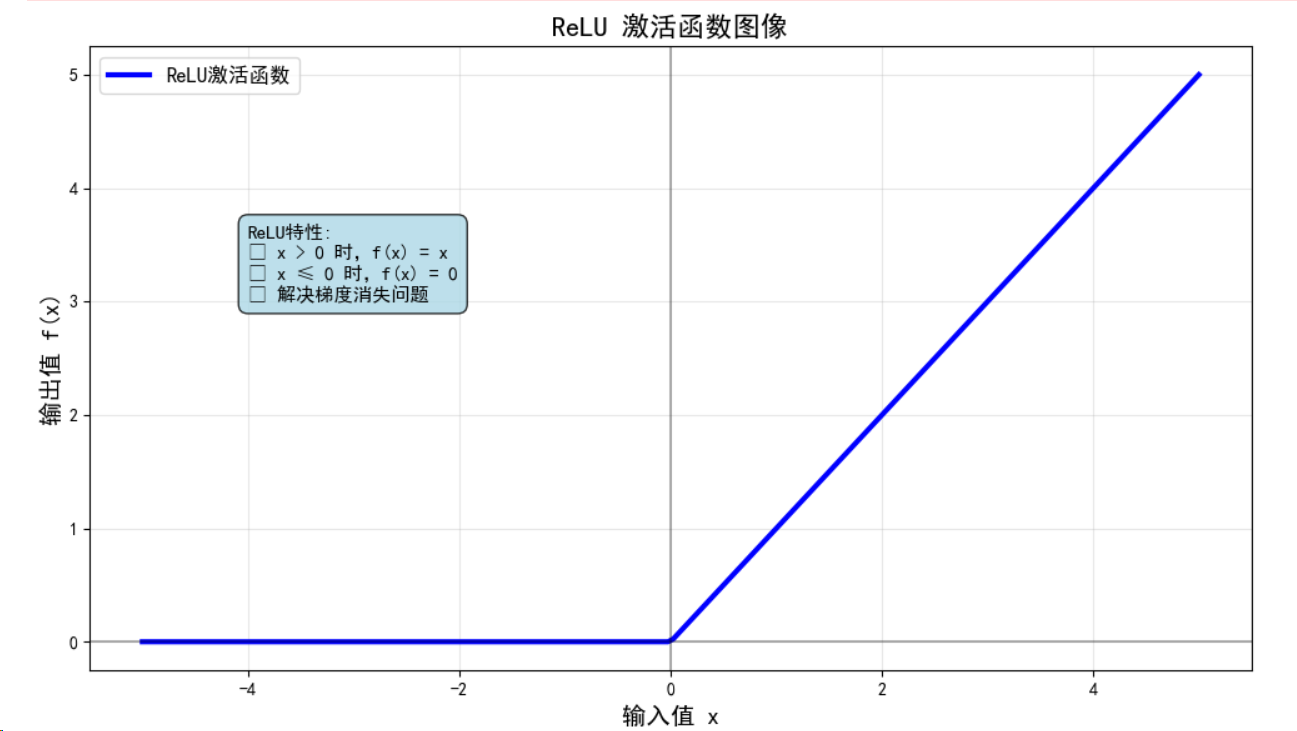
2.1 ReLU (Rectified Linear Unit)

数学定义：f(x) = max(0, x)

特点：

• 简单高效，计算速度快
• 解决梯度消失问题
• 可能导致神经元"死亡"

import torch
import torch.nn as nn
import torch.nn.functional as F
import matplotlib.pyplot as plt
import numpy as np
import seaborn as sns
from matplotlib.gridspec import GridSpec# 设置matplotlib中文显示和样式
plt.rcParams['font.sans-serif'] = ['SimHei', 'DejaVu Sans']
plt.rcParams['axes.unicode_minus'] = False
plt.style.use('seaborn-v0_8')
sns.set_palette("husl")# 设备选择函数
def get_device():if torch.cuda.is_available():device = torch.device('cuda')print(f"使用GPU: {torch.cuda.get_device_name(0)}")else:device = torch.device('cpu')print("使用CPU")return devicedevice = get_device()# ReLU激活函数演示
class ReLUDemo(nn.Module):def __init__(self):super(ReLUDemo, self).__init__()self.relu = nn.ReLU()def forward(self, x):return self.relu(x)# 创建测试数据
x = torch.linspace(-5, 5, 100).to(device)
relu_demo = ReLUDemo().to(device)# 计算ReLU输出
with torch.no_grad():y_relu = relu_demo(x)print("ReLU函数特性:")
print(f"输入范围: [{x.min():.2f}, {x.max():.2f}]")
print(f"输出范围: [{y_relu.min():.2f}, {y_relu.max():.2f}]")# 可视化ReLU函数
def plot_activation_function(x, y, title, ax=None):"""绘制激活函数"""if ax is None:plt.figure(figsize=(8, 6))ax = plt.gca()x_np = x.cpu().numpy()y_np = y.cpu().numpy()ax.plot(x_np, y_np, linewidth=3, label=title)ax.grid(True, alpha=0.3)ax.set_xlabel('输入值 (x)', fontsize=12)ax.set_ylabel('输出值 f(x)', fontsize=12)ax.set_title(f'{title} 激活函数', fontsize=14, fontweight='bold')ax.legend(fontsize=11)return ax# 绘制ReLU
plot_activation_function(x, y_relu, 'ReLU')
plt.tight_layout()
plt.show()

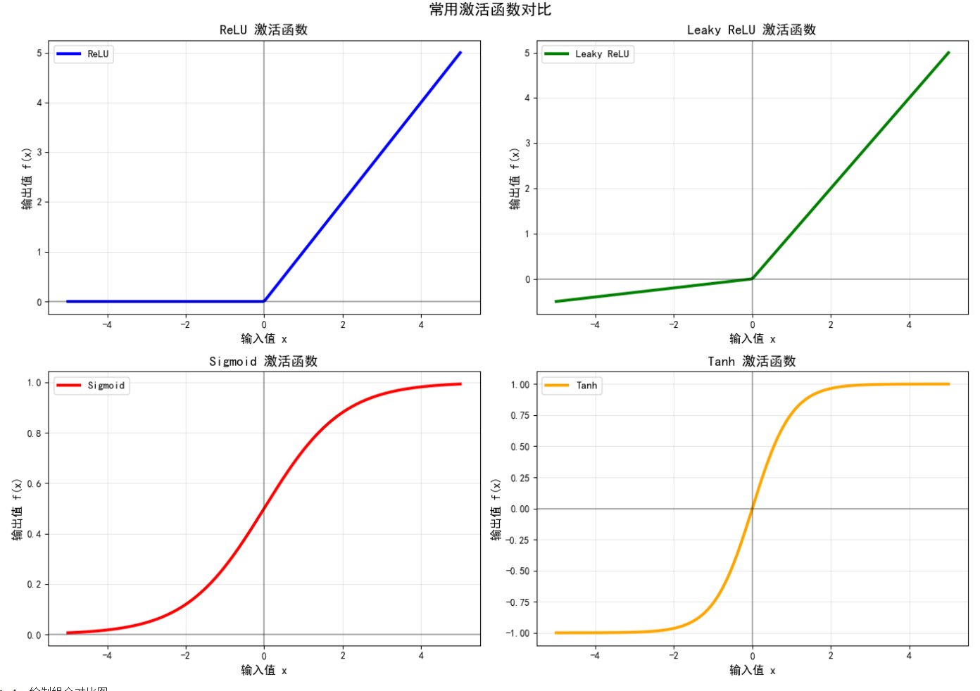
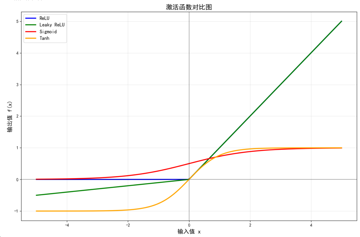
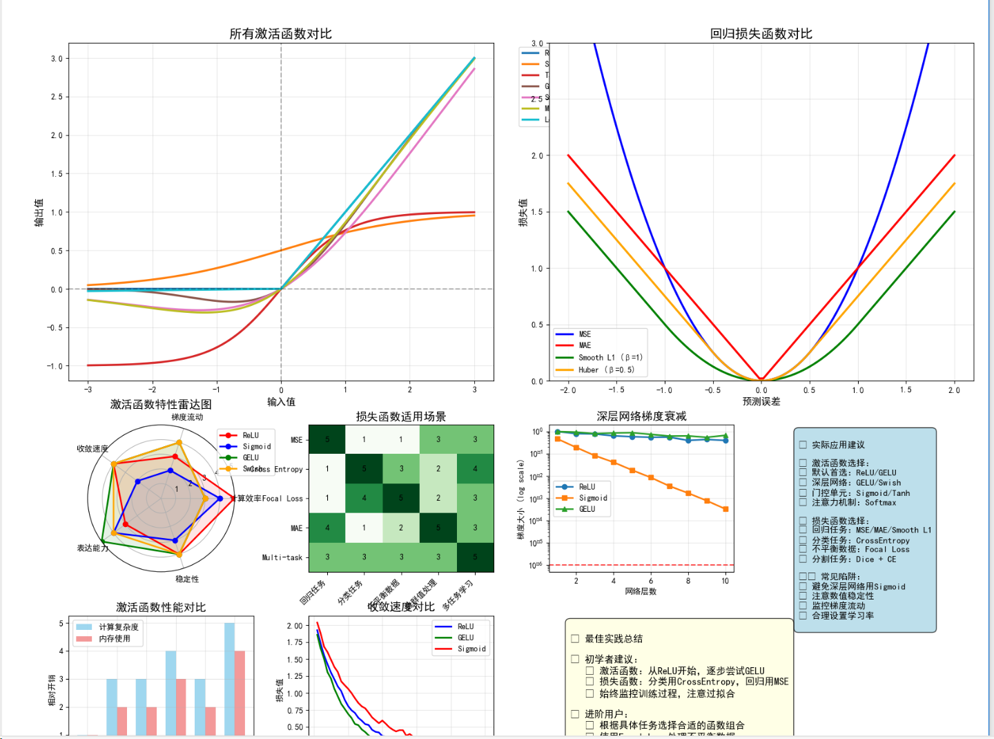
ReLU : 非负区间线性，负区间为0，计算简单，解决梯度消失
Leaky ReLU : 负区间有小斜率，避免神经元死亡问题
Sigmoid : 输出在(0,1)区间，常用于二分类输出层
Tanh : 输出在(-1,1)区间，比Sigmoid收敛更快

import torch
import torch.nn as nn
import matplotlib.pyplot as plt
import numpy as np
import platform# 强制解决中文显示问题
def force_chinese_font():"""强制设置中文字体 - 最简单有效的方法"""import matplotlib# 清空现有设置matplotlib.rcdefaults()# 根据操作系统强制设置字体system = platform.system()if system == 'Windows':plt.rcParams['font.sans-serif'] = ['Microsoft YaHei', 'SimHei']elif system == 'Darwin':  # macOSplt.rcParams['font.sans-serif'] = ['PingFang SC', 'Arial Unicode MS']else:  # Linuxplt.rcParams['font.sans-serif'] = ['DejaVu Sans']plt.rcParams['axes.unicode_minus'] = False# 强制更新matplotlib.font_manager._rebuild()print(f"✓ 字体设置完成: {plt.rcParams['font.sans-serif'][0]}")# 立即设置字体
print("=== 强制设置中文字体 ===")
try:force_chinese_font()
except:# 如果上面的方法失败，使用最基本的设置plt.rcParams['font.sans-serif'] = ['SimHei', 'Microsoft YaHei', 'DejaVu Sans']plt.rcParams['axes.unicode_minus'] = Falseprint("✓ 使用备用字体设置")# 设备选择
device = torch.device('cuda' if torch.cuda.is_available() else 'cpu')
print(f"✓ 使用设备: {device}")# 激活函数类
class ActivationDemo(nn.Module):def __init__(self):super().__init__()self.relu = nn.ReLU()self.leaky_relu = nn.LeakyReLU(0.1)self.sigmoid = nn.Sigmoid()self.tanh = nn.Tanh()def forward(self, x, func_type='relu'):if func_type == 'relu':return self.relu(x)elif func_type == 'leaky_relu':return self.leaky_relu(x)elif func_type == 'sigmoid':return self.sigmoid(x)elif func_type == 'tanh':return self.tanh(x)# 创建数据
x = torch.linspace(-5, 5, 200).to(device)
model = ActivationDemo().to(device)print(f"\n=== 计算激活函数 ===")
print(f"输入范围: [{x.min():.2f}, {x.max():.2f}]")# 计算各种激活函数
activations = {}
func_names = ['relu', 'leaky_relu', 'sigmoid', 'tanh']
chinese_names = ['ReLU', 'Leaky ReLU', 'Sigmoid', 'Tanh']with torch.no_grad():for func, name in zip(func_names, chinese_names):y = model(x, func)activations[name] = (x.cpu().numpy(), y.cpu().numpy())print(f"{name:12} 输出范围: [{y.min():.3f}, {y.max():.3f}]")# 绘制单个激活函数图
def plot_single_activation():"""绘制ReLU激活函数"""plt.figure(figsize=(10, 6))x_np, y_np = activations['ReLU']plt.plot(x_np, y_np, 'b-', linewidth=3, label='ReLU激活函数')plt.axhline(y=0, color='k', linestyle='-', alpha=0.3)plt.axvline(x=0, color='k', linestyle='-', alpha=0.3)plt.grid(True, alpha=0.3)plt.xlabel('输入值 x', fontsize=14)plt.ylabel('输出值 f(x)', fontsize=14)plt.title('ReLU 激活函数图像', fontsize=16, fontweight='bold')plt.legend(fontsize=12)# 添加函数特性说明plt.text(-4, 3, 'ReLU特性:\n• x > 0 时，f(x) = x\n• x ≤ 0 时，f(x) = 0\n• 解决梯度消失问题', fontsize=11, bbox=dict(boxstyle="round,pad=0.5", facecolor="lightblue", alpha=0.8))plt.tight_layout()plt.show()# 绘制所有激活函数对比
def plot_all_activations():"""绘制所有激活函数对比"""fig, axes = plt.subplots(2, 2, figsize=(14, 10))axes = axes.flatten()colors = ['blue', 'green', 'red', 'orange']for i, (name, color) in enumerate(zip(chinese_names, colors)):ax = axes[i]x_np, y_np = activations[name]ax.plot(x_np, y_np, color=color, linewidth=3, label=name)ax.axhline(y=0, color='k', linestyle='-', alpha=0.3)ax.axvline(x=0, color='k', linestyle='-', alpha=0.3)ax.grid(True, alpha=0.3)ax.set_xlabel('输入值 x', fontsize=12)ax.set_ylabel('输出值 f(x)', fontsize=12)ax.set_title(f'{name} 激活函数', fontsize=14, fontweight='bold')ax.legend(fontsize=11)plt.suptitle('常用激活函数对比', fontsize=16, fontweight='bold')plt.tight_layout()plt.show()# 绘制组合对比图
def plot_combined():"""在一张图中对比所有激活函数"""plt.figure(figsize=(12, 8))colors = ['blue', 'green', 'red', 'orange']for (name, color) in zip(chinese_names, colors):x_np, y_np = activations[name]plt.plot(x_np, y_np, color=color, linewidth=2.5, label=name)plt.axhline(y=0, color='k', linestyle='-', alpha=0.3)plt.axvline(x=0, color='k', linestyle='-', alpha=0.3)plt.grid(True, alpha=0.3)plt.xlabel('输入值 x', fontsize=14)plt.ylabel('输出值 f(x)', fontsize=14)plt.title('激活函数对比图', fontsize=16, fontweight='bold')plt.legend(fontsize=12, loc='upper left')plt.tight_layout()plt.show()# 测试中文显示
def test_chinese():"""测试中文字体显示"""plt.figure(figsize=(8, 4))plt.text(0.5, 0.7, '中文测试：PyTorch激活函数', fontsize=20, ha='center', fontweight='bold')plt.text(0.5, 0.5, '神经网络 • 深度学习 • 人工智能', fontsize=16, ha='center')plt.text(0.5, 0.3, '数学符号：α β γ δ ∑ ∏ ∫ ∂', fontsize=14, ha='center')plt.xlim(0, 1)plt.ylim(0, 1)plt.axis('off')plt.title('中文字体显示测试', fontsize=16)plt.tight_layout()plt.show()# 执行绘图
print("\n=== 开始绘制图形 ===")# 1. 测试中文显示
print("1. 测试中文字体显示...")
test_chinese()# 2. 绘制ReLU单独图
print("2. 绘制ReLU激活函数...")
plot_single_activation()# 3. 绘制所有激活函数分别展示
print("3. 绘制所有激活函数对比...")
plot_all_activations()# 4. 绘制组合对比图
print("4. 绘制组合对比图...")
plot_combined()# 激活函数特性分析
print("\n=== 激活函数特性分析 ===")
analysis = {'ReLU': '非负区间线性，负区间为0，计算简单，解决梯度消失','Leaky ReLU': '负区间有小斜率，避免神经元死亡问题','Sigmoid': '输出在(0,1)区间，常用于二分类输出层','Tanh': '输出在(-1,1)区间，比Sigmoid收敛更快'
}for name, desc in analysis.items():print(f"{name:12}: {desc}")print(f"\n=== 系统信息 ===")
print(f"PyTorch版本: {torch.__version__}")
print(f"设备: {device}")
print(f"字体设置: {plt.rcParams['font.sans-serif'][0]}")
print("\n✅ 所有任务完成！中文显示应该正常了！")

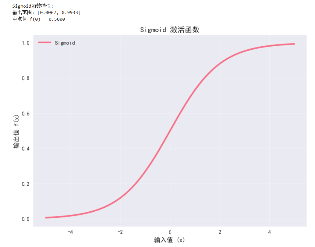
2.2 Sigmoid函数

数学定义：f(x) = 1/(1 + e^(-x))

特点：

• 输出范围(0,1)，适合二分类
• 存在梯度消失问题
• 输出不以零为中心

# Sigmoid激活函数演示
class SigmoidDemo(nn.Module):def __init__(self):super(SigmoidDemo, self).__init__()self.sigmoid = nn.Sigmoid()def forward(self, x):return self.sigmoid(x)sigmoid_demo = SigmoidDemo().to(device)with torch.no_grad():y_sigmoid = sigmoid_demo(x)print("\nSigmoid函数特性:")
print(f"输出范围: [{y_sigmoid.min():.4f}, {y_sigmoid.max():.4f}]")
print(f"中点值 f(0) = {sigmoid_demo(torch.tensor(0.0).to(device)):.4f}")# 可视化Sigmoid函数
plot_activation_function(x, y_sigmoid, 'Sigmoid')
plt.tight_layout()
plt.show()

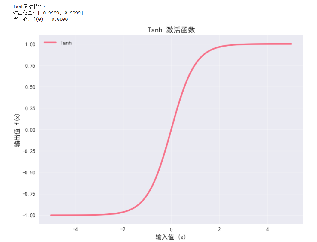
2.3 Tanh函数

数学定义：f(x) = (e^x - e^(-x))/(ex + e^(-x))

特点：

• 输出范围(-1,1)，以零为中心
• 比Sigmoid收敛更快
• 仍有梯度消失问题

# Tanh激活函数演示
class TanhDemo(nn.Module):def __init__(self):super(TanhDemo, self).__init__()self.tanh = nn.Tanh()def forward(self, x):return self.tanh(x)tanh_demo = TanhDemo().to(device)with torch.no_grad():y_tanh = tanh_demo(x)print("\nTanh函数特性:")
print(f"输出范围: [{y_tanh.min():.4f}, {y_tanh.max():.4f}]")
print(f"零中心: f(0) = {tanh_demo(torch.tensor(0.0).to(device)):.4f}")# 可视化Tanh函数
plot_activation_function(x, y_tanh, 'Tanh')
plt.tight_layout()
plt.show()

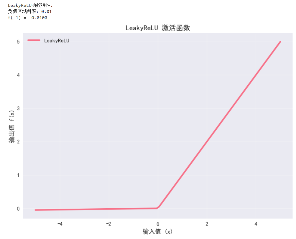
2.4 LeakyReLU

数学定义：f(x) = max(αx, x)，其中α是小的正数（通常0.01）

特点：

• 解决ReLU的"死亡"问题
• 保持ReLU的优点

# LeakyReLU激活函数演示
class LeakyReLUDemo(nn.Module):def __init__(self, negative_slope=0.01):super(LeakyReLUDemo, self).__init__()self.leaky_relu = nn.LeakyReLU(negative_slope=negative_slope)def forward(self, x):return self.leaky_relu(x)leaky_relu_demo = LeakyReLUDemo().to(device)with torch.no_grad():y_leaky_relu = leaky_relu_demo(x)print("\nLeakyReLU函数特性:")
print(f"负值区域斜率: 0.01")
print(f"f(-1) = {leaky_relu_demo(torch.tensor(-1.0).to(device)):.4f}")# 可视化LeakyReLU函数
plot_activation_function(x, y_leaky_relu, 'LeakyReLU')
plt.tight_layout()
plt.show()

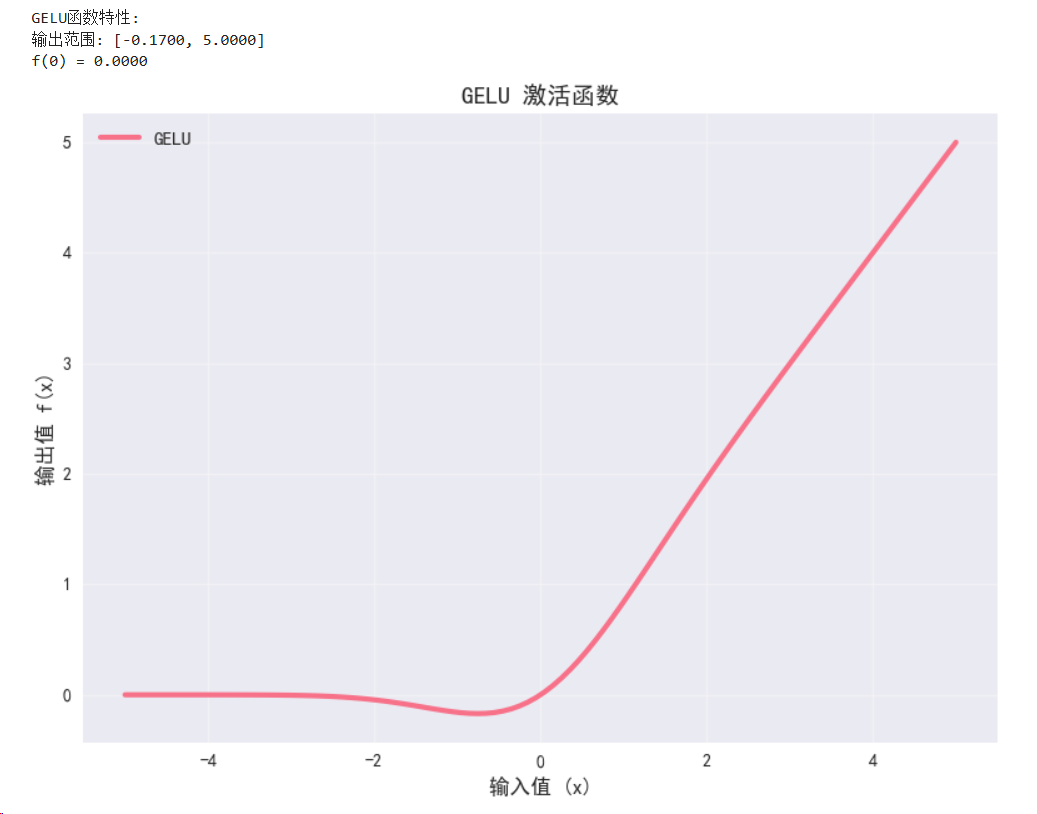
2.5 GELU (Gaussian Error Linear Unit)

数学定义：f(x) = x * Φ(x)，其中Φ(x)是标准高斯分布的累积分布函数

特点：

• Transformer模型中广泛使用
• 平滑的激活函数
• 性能优于ReLU

# GELU激活函数演示
class GELUDemo(nn.Module):def __init__(self):super(GELUDemo, self).__init__()self.gelu = nn.GELU()def forward(self, x):return self.gelu(x)gelu_demo = GELUDemo().to(device)with torch.no_grad():y_gelu = gelu_demo(x)print("\nGELU函数特性:")
print(f"输出范围: [{y_gelu.min():.4f}, {y_gelu.max():.4f}]")
print(f"f(0) = {gelu_demo(torch.tensor(0.0).to(device)):.4f}")# 可视化GELU函数
plot_activation_function(x, y_gelu, 'GELU')
plt.tight_layout()
plt.show()

3. 激活函数的梯度分析

import torch
import torch.nn.functional as F
import matplotlib.pyplot as plt
import numpy as np# 设置中文字体支持
plt.rcParams['font.sans-serif'] = ['SimHei', 'DejaVu Sans']
plt.rcParams['axes.unicode_minus'] = False# 检查设备
device = torch.device('cuda' if torch.cuda.is_available() else 'cpu')
print(f"使用设备: {device}")# 修复的梯度计算函数
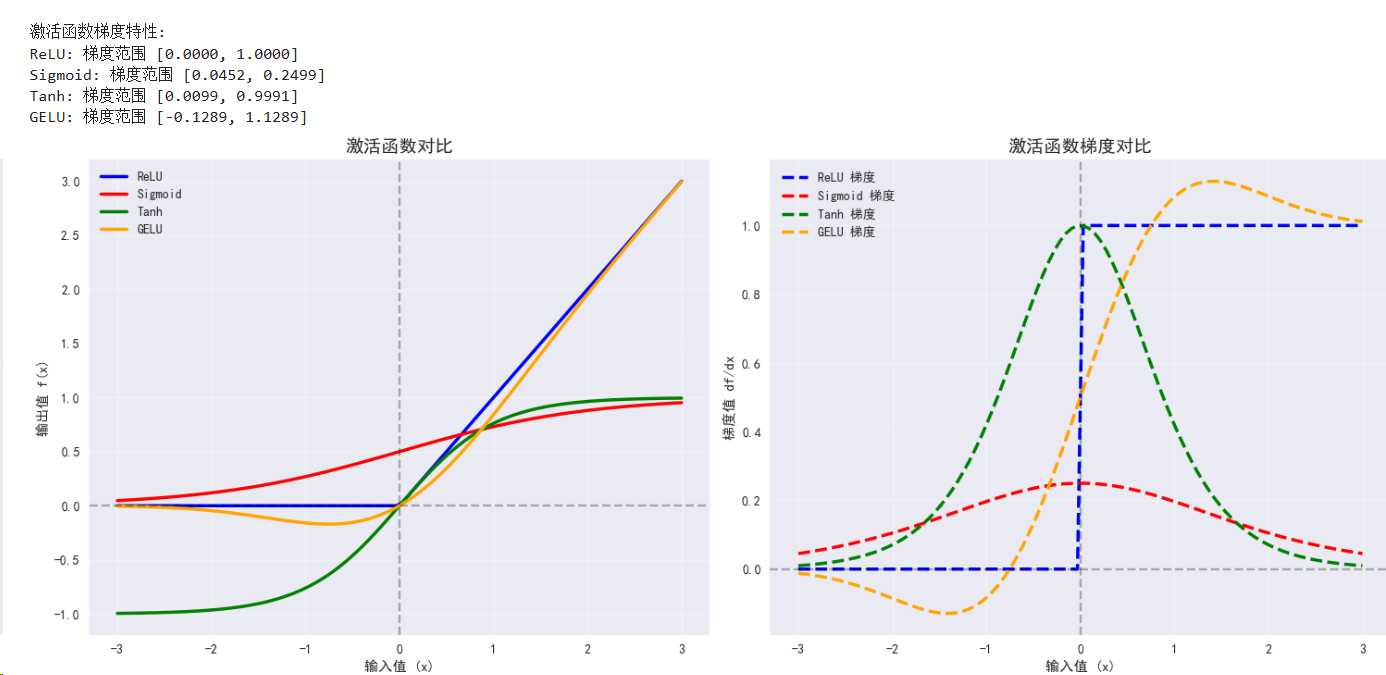
def compute_gradients():"""计算不同激活函数的梯度"""# 定义激活函数functions = {'ReLU': F.relu,'Sigmoid': torch.sigmoid,'Tanh': torch.tanh,'GELU': F.gelu}gradients = {}outputs = {}# 为每个函数单独创建输入张量for name, func in functions.items():# 每次都创建新的张量，确保requires_grad=Truex = torch.linspace(-3, 3, 100, requires_grad=True, device=device)# 计算函数输出y = func(x)# 计算梯度（对每个输出点求和后反向传播）y_sum = y.sum()y_sum.backward()# 保存梯度和输出gradients[name] = x.grad.clone().detach()# 重新计算输出用于可视化（不需要梯度）with torch.no_grad():x_no_grad = torch.linspace(-3, 3, 100, device=device)outputs[name] = func(x_no_grad)# 返回x轴坐标用于绘图x_axis = torch.linspace(-3, 3, 100, device=device)return x_axis, gradients, outputs# 执行梯度计算
x_grad, gradients, outputs = compute_gradients()print("\n激活函数梯度特性:")
for name, grad in gradients.items():print(f"{name}: 梯度范围 [{grad.min():.4f}, {grad.max():.4f}]")# 可视化激活函数对比
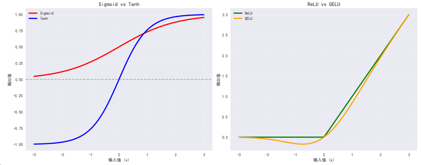
def plot_activation_comparison():"""绘制多个激活函数的对比图"""fig, ((ax1, ax2), (ax3, ax4)) = plt.subplots(2, 2, figsize=(15, 12))x_np = x_grad.cpu().numpy()# 子图1: 所有激活函数colors = ['blue', 'red', 'green', 'orange']for i, (name, y) in enumerate(outputs.items()):y_np = y.cpu().numpy()ax1.plot(x_np, y_np, linewidth=2.5, label=name, color=colors[i])ax1.set_title('激活函数对比', fontsize=14, fontweight='bold')ax1.set_xlabel('输入值 (x)')ax1.set_ylabel('输出值 f(x)')ax1.grid(True, alpha=0.3)ax1.legend()ax1.axhline(y=0, color='k', linestyle='--', alpha=0.3)ax1.axvline(x=0, color='k', linestyle='--', alpha=0.3)# 子图2: 梯度对比for i, (name, grad) in enumerate(gradients.items()):grad_np = grad.cpu().numpy()ax2.plot(x_np, grad_np, linewidth=2.5, label=f"{name} 梯度", linestyle='--', color=colors[i])ax2.set_title('激活函数梯度对比', fontsize=14, fontweight='bold')ax2.set_xlabel('输入值 (x)')ax2.set_ylabel('梯度值 df/dx')ax2.grid(True, alpha=0.3)ax2.legend()ax2.axhline(y=0, color='k', linestyle='--', alpha=0.3)ax2.axvline(x=0, color='k', linestyle='--', alpha=0.3)# 子图3: Sigmoid vs Tanhsigmoid_y = outputs['Sigmoid'].cpu().numpy()tanh_y = outputs['Tanh'].cpu().numpy()ax3.plot(x_np, sigmoid_y, linewidth=3, label='Sigmoid', color='red')ax3.plot(x_np, tanh_y, linewidth=3, label='Tanh', color='blue')ax3.set_title('Sigmoid vs Tanh', fontsize=14, fontweight='bold')ax3.set_xlabel('输入值 (x)')ax3.set_ylabel('输出值')ax3.grid(True, alpha=0.3)ax3.legend()ax3.axhline(y=0, color='k', linestyle='--', alpha=0.3)# 子图4: ReLU vs GELUrelu_y = outputs['ReLU'].cpu().numpy()gelu_y = outputs['GELU'].cpu().numpy()ax4.plot(x_np, relu_y, linewidth=3, label='ReLU', color='green')ax4.plot(x_np, gelu_y, linewidth=3, label='GELU', color='orange')ax4.set_title('ReLU vs GELU', fontsize=14, fontweight='bold')ax4.set_xlabel('输入值 (x)')ax4.set_ylabel('输出值')ax4.grid(True, alpha=0.3)ax4.legend()plt.tight_layout()plt.show()# 执行可视化
plot_activation_comparison()# 梯度饱和分析
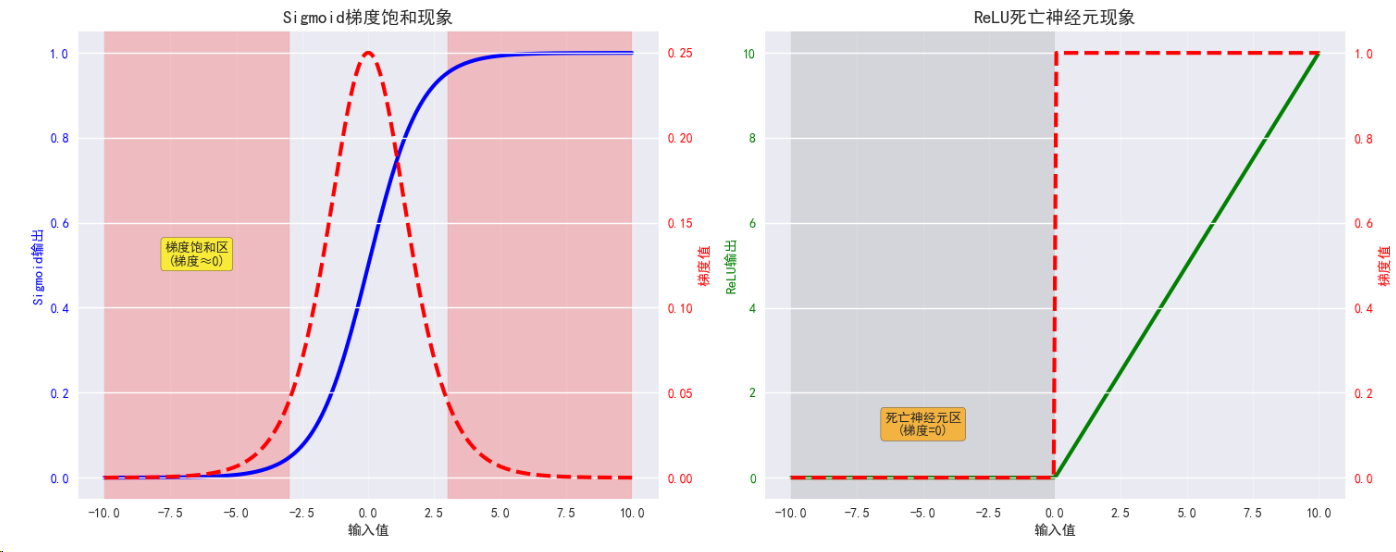
def plot_gradient_saturation():"""分析梯度饱和现象"""fig, (ax1, ax2) = plt.subplots(1, 2, figsize=(15, 6))# 创建更大范围的输入用于观察饱和现象x_sat = torch.linspace(-10, 10, 200, requires_grad=True, device=device)# Sigmoid梯度饱和分析sigmoid_out = torch.sigmoid(x_sat)sigmoid_out.sum().backward()sigmoid_grad = x_sat.grad.clone()x_np = x_sat.detach().cpu().numpy()sigmoid_np = sigmoid_out.detach().cpu().numpy()sigmoid_grad_np = sigmoid_grad.cpu().numpy()# 绘制Sigmoid函数和其梯度ax1_twin = ax1.twinx()line1 = ax1.plot(x_np, sigmoid_np, 'b-', linewidth=3, label='Sigmoid输出')ax1.set_ylabel('Sigmoid输出', color='b')ax1.tick_params(axis='y', labelcolor='b')line2 = ax1_twin.plot(x_np, sigmoid_grad_np, 'r--', linewidth=3, label='梯度')ax1_twin.set_ylabel('梯度值', color='r')ax1_twin.tick_params(axis='y', labelcolor='r')ax1.set_xlabel('输入值')ax1.set_title('Sigmoid梯度饱和现象', fontsize=14, fontweight='bold')ax1.grid(True, alpha=0.3)# 添加饱和区域标注ax1.axvspan(-10, -3, alpha=0.2, color='red', label='饱和区')ax1.axvspan(3, 10, alpha=0.2, color='red')ax1.text(-6.5, 0.5, '梯度饱和区\n(梯度≈0)', fontsize=10, ha='center',bbox=dict(boxstyle="round,pad=0.3", facecolor="yellow", alpha=0.7))# ReLU死亡神经元分析# 重新创建张量用于ReLU分析x_relu = torch.linspace(-10, 10, 200, requires_grad=True, device=device)relu_out = F.relu(x_relu)relu_out.sum().backward()relu_grad = x_relu.grad.clone()relu_np = relu_out.detach().cpu().numpy()relu_grad_np = relu_grad.cpu().numpy()ax2_twin = ax2.twinx()line3 = ax2.plot(x_np, relu_np, 'g-', linewidth=3, label='ReLU输出')ax2.set_ylabel('ReLU输出', color='g')ax2.tick_params(axis='y', labelcolor='g')line4 = ax2_twin.plot(x_np, relu_grad_np, 'r--', linewidth=3, label='梯度')ax2_twin.set_ylabel('梯度值', color='r')ax2_twin.tick_params(axis='y', labelcolor='r')ax2.set_xlabel('输入值')ax2.set_title('ReLU死亡神经元现象', fontsize=14, fontweight='bold')ax2.grid(True, alpha=0.3)# 添加死亡区域标注ax2.axvspan(-10, 0, alpha=0.2, color='gray', label='死亡区')ax2.text(-5, 1, '死亡神经元区\n(梯度=0)', fontsize=10, ha='center',bbox=dict(boxstyle="round,pad=0.3", facecolor="orange", alpha=0.7))plt.tight_layout()plt.show()# 执行梯度饱和分析
plot_gradient_saturation()# 打印激活函数特性总结
def print_activation_summary():"""打印激活函数特性总结"""print("\n" + "="*60)print("激活函数特性总结")print("="*60)print("\n1. ReLU (Rectified Linear Unit)")print("   - 优点: 计算简单，缓解梯度饱和，稀疏激活")print("   - 缺点: 死亡神经元问题，输出不以零为中心")print("   - 适用: 隐藏层，特别是深度网络")print("\n2. Sigmoid")print("   - 优点: 平滑函数，输出在(0,1)之间")print("   - 缺点: 梯度饱和严重，输出不以零为中心")print("   - 适用: 二分类输出层")print("\n3. Tanh")print("   - 优点: 输出以零为中心，比Sigmoid梯度饱和稍好")print("   - 缺点: 仍有梯度饱和问题")print("   - 适用: 隐藏层，特别是RNN")print("\n4. GELU (Gaussian Error Linear Unit)")print("   - 优点: 平滑函数，性能优异，适合Transformer")print("   - 缺点: 计算复杂度较高")print("   - 适用: 现代深度学习模型，特别是Transformer")print_activation_summary()

1. ReLU (Rectified Linear Unit)

   • 优点: 计算简单，缓解梯度饱和，稀疏激活
   • 缺点: 死亡神经元问题，输出不以零为中心
   • 适用: 隐藏层，特别是深度网络

2. Sigmoid

   • 优点: 平滑函数，输出在(0,1)之间
   • 缺点: 梯度饱和严重，输出不以零为中心
   • 适用: 二分类输出层

3. Tanh

   • 优点: 输出以零为中心，比Sigmoid梯度饱和稍好
   • 缺点: 仍有梯度饱和问题
   • 适用: 隐藏层，特别是RNN

4. GELU (Gaussian Error Linear Unit)

   • 优点: 平滑函数，性能优异，适合Transformer
   • 缺点: 计算复杂度较高
   • 适用: 现代深度学习模型，特别是Transformer

损失函数详解

1. 什么是损失函数？

损失函数（Loss Function）用于衡量模型预测值与真实值之间的差异。它是优化算法的指导方向，决定了模型的学习目标。

2. 回归任务损失函数

2.1 均方误差损失 (MSE Loss)

数学定义：L = (1/n) * Σ(yi - ŷi)²

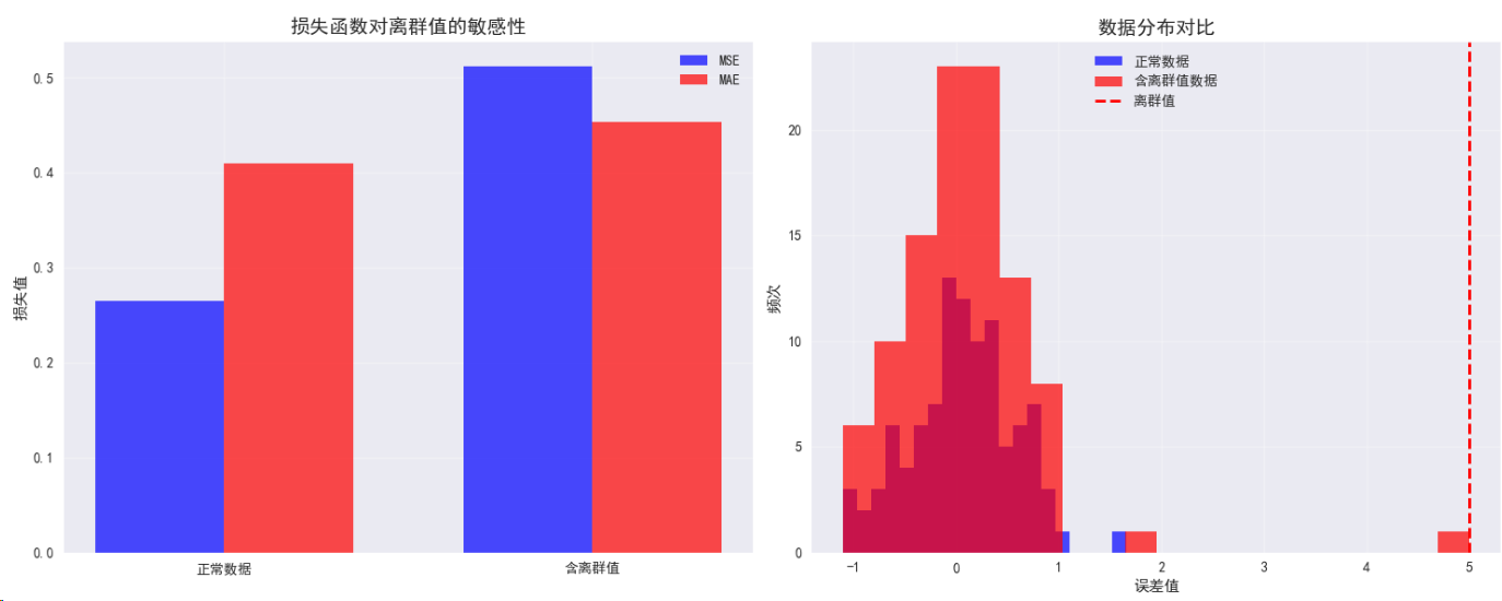
特点：

• 对离群值敏感
• 梯度随误差增大而增大
• 适用于回归任务

# MSE Loss演示
class MSELossDemo:def __init__(self, device):self.device = deviceself.mse_loss = nn.MSELoss()def demonstrate(self):# 创建示例数据y_true = torch.randn(100, 1).to(self.device)y_pred = y_true + 0.1 * torch.randn(100, 1).to(self.device)  # 添加噪声# 计算损失loss = self.mse_loss(y_pred, y_true)print(f"\nMSE Loss演示:")print(f"真实值范围: [{y_true.min():.4f}, {y_true.max():.4f}]")print(f"预测值范围: [{y_pred.min():.4f}, {y_pred.max():.4f}]")print(f"MSE Loss: {loss.item():.6f}")return lossmse_demo = MSELossDemo(device)
mse_loss = mse_demo.demonstrate()# 可视化损失函数特性
def plot_loss_functions():"""可视化不同损失函数的特性"""fig, ((ax1, ax2), (ax3, ax4)) = plt.subplots(2, 2, figsize=(15, 12))# 创建误差范围errors = torch.linspace(-3, 3, 100)# MSE Lossmse_losses = errors ** 2ax1.plot(errors.numpy(), mse_losses.numpy(), 'b-', linewidth=3, label='MSE Loss')ax1.set_title('均方误差损失 (MSE)', fontsize=14, fontweight='bold')ax1.set_xlabel('预测误差')ax1.set_ylabel('损失值')ax1.grid(True, alpha=0.3)ax1.legend()# MAE Lossmae_losses = torch.abs(errors)ax2.plot(errors.numpy(), mae_losses.numpy(), 'r-', linewidth=3, label='MAE Loss')ax2.set_title('平均绝对误差损失 (MAE)', fontsize=14, fontweight='bold')ax2.set_xlabel('预测误差')ax2.set_ylabel('损失值')ax2.grid(True, alpha=0.3)ax2.legend()# Smooth L1 Lossbeta = 1.0smooth_l1_losses = torch.where(torch.abs(errors) < beta,0.5 * errors ** 2 / beta,torch.abs(errors) - 0.5 * beta)ax3.plot(errors.numpy(), smooth_l1_losses.numpy(), 'g-', linewidth=3, label='Smooth L1')ax3.set_title(f'Smooth L1 损失 (β={beta})', fontsize=14, fontweight='bold')ax3.set_xlabel('预测误差')ax3.set_ylabel('损失值')ax3.grid(True, alpha=0.3)ax3.legend()# 对比所有回归损失ax4.plot(errors.numpy(), mse_losses.numpy(), 'b-', linewidth=2, label='MSE')ax4.plot(errors.numpy(), mae_losses.numpy(), 'r-', linewidth=2, label='MAE')ax4.plot(errors.numpy(), smooth_l1_losses.numpy(), 'g-', linewidth=2, label='Smooth L1')ax4.set_title('回归损失函数对比', fontsize=14, fontweight='bold')ax4.set_xlabel('预测误差')ax4.set_ylabel('损失值')ax4.grid(True, alpha=0.3)ax4.legend()ax4.set_ylim(0, 5)  # 限制y轴范围以便观察plt.tight_layout()plt.show()# 离群值敏感性分析fig, (ax1, ax2) = plt.subplots(1, 2, figsize=(15, 6))# 正常数据 vs 含离群值数据normal_errors = torch.randn(100) * 0.5outlier_errors = normal_errors.clone()outlier_errors[0] = 5.0  # 添加离群值# MSE对离群值的敏感性mse_normal = (normal_errors ** 2).mean()mse_outlier = (outlier_errors ** 2).mean()# MAE对离群值的敏感性mae_normal = torch.abs(normal_errors).mean()mae_outlier = torch.abs(outlier_errors).mean()losses = ['正常数据', '含离群值']mse_values = [mse_normal.item(), mse_outlier.item()]mae_values = [mae_normal.item(), mae_outlier.item()]x_pos = np.arange(len(losses))width = 0.35ax1.bar(x_pos - width/2, mse_values, width, label='MSE', color='blue', alpha=0.7)ax1.bar(x_pos + width/2, mae_values, width, label='MAE', color='red', alpha=0.7)ax1.set_title('损失函数对离群值的敏感性', fontsize=14, fontweight='bold')ax1.set_ylabel('损失值')ax1.set_xticks(x_pos)ax1.set_xticklabels(losses)ax1.legend()ax1.grid(True, alpha=0.3)# 数据分布可视化ax2.hist(normal_errors.numpy(), bins=20, alpha=0.7, label='正常数据', color='blue')ax2.hist(outlier_errors.numpy(), bins=20, alpha=0.7, label='含离群值数据', color='red')ax2.axvline(x=5.0, color='red', linestyle='--', linewidth=2, label='离群值')ax2.set_title('数据分布对比', fontsize=14, fontweight='bold')ax2.set_xlabel('误差值')ax2.set_ylabel('频次')ax2.legend()ax2.grid(True, alpha=0.3)plt.tight_layout()plt.show()plot_loss_functions()

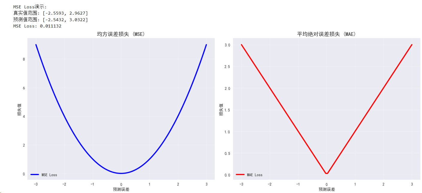
2.2 平均绝对误差损失 (MAE Loss)

数学定义：L = (1/n) * Σ|yi - ŷi|

特点：

• 对离群值不敏感
• 梯度恒定
• 更稳健的回归损失

# MAE Loss演示
class MAELossDemo:def __init__(self, device):self.device = deviceself.mae_loss = nn.L1Loss()def demonstrate(self):# 创建包含离群值的数据y_true = torch.randn(100, 1).to(self.device)y_pred = y_true + 0.1 * torch.randn(100, 1).to(self.device)# 添加离群值y_pred[0] = y_true[0] + 5.0  # 人为添加大误差# 比较MSE和MAEmse_loss = nn.MSELoss()(y_pred, y_true)mae_loss = self.mae_loss(y_pred, y_true)print(f"\n对比MSE和MAE对离群值的敏感性:")print(f"MSE Loss: {mse_loss.item():.6f}")print(f"MAE Loss: {mae_loss.item():.6f}")print(f"MSE/MAE比值: {(mse_loss/mae_loss).item():.2f}")return mae_lossmae_demo = MAELossDemo(device)
mae_loss = mae_demo.demonstrate()

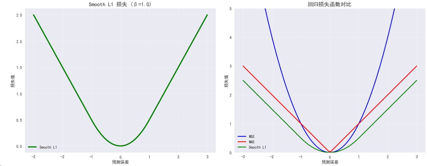
2.3 Smooth L1 Loss (Huber Loss)

数学定义：

• 当|x| < β时：L = 0.5 * x² / β
• 当|x| ≥ β时：L = |x| - 0.5 * β

特点：

• 结合MSE和MAE的优点
• 对离群值相对稳健
• 梯度变化平滑

# Smooth L1 Loss演示
class SmoothL1LossDemo:def __init__(self, device, beta=1.0):self.device = deviceself.smooth_l1_loss = nn.SmoothL1Loss(beta=beta)self.beta = betadef demonstrate(self):# 创建不同误差程度的数据errors = torch.tensor([-3, -1, -0.5, 0, 0.5, 1, 3], dtype=torch.float32).to(self.device)y_true = torch.zeros_like(errors)y_pred = errors# 计算不同损失函数的值smooth_l1 = self.smooth_l1_loss(y_pred, y_true)mse = nn.MSELoss()(y_pred, y_true)mae = nn.L1Loss()(y_pred, y_true)print(f"\nSmooth L1 Loss特性分析 (β={self.beta}):")print("误差值\t| Smooth L1\t| MSE\t\t| MAE")print("-" * 50)for i, error in enumerate(errors):single_error = error.unsqueeze(0)zero = torch.zeros_like(single_error)s_l1 = self.smooth_l1_loss(single_error, zero).item()mse_val = nn.MSELoss()(single_error, zero).item()mae_val = nn.L1Loss()(single_error, zero).item()print(f"{error.item():6.1f}\t| {s_l1:8.4f}\t| {mse_val:8.4f}\t| {mae_val:8.4f}")return smooth_l1smooth_l1_demo = SmoothL1LossDemo(device)
smooth_l1_loss = smooth_l1_demo.demonstrate()# 可视化Smooth L1 Loss的特性
def plot_smooth_l1_analysis():"""分析Smooth L1 Loss在不同β值下的行为"""fig, (ax1, ax2) = plt.subplots(1, 2, figsize=(15, 6))errors = torch.linspace(-3, 3, 100)betas = [0.5, 1.0, 2.0]colors = ['red', 'blue', 'green']# 不同β值的Smooth L1 Lossfor beta, color in zip(betas, colors):smooth_l1_losses = torch.where(torch.abs(errors) < beta,0.5 * errors ** 2 / beta,torch.abs(errors) - 0.5 * beta)ax1.plot(errors.numpy(), smooth_l1_losses.numpy(), color=color, linewidth=3, label=f'β={beta}')# 添加MSE和MAE作为参考mse_losses = errors ** 2mae_losses = torch.abs(errors)ax1.plot(errors.numpy(), mse_losses.numpy(), 'k--', linewidth=2, alpha=0.5, label='MSE (参考)')ax1.plot(errors.numpy(), mae_losses.numpy(), 'k:', linewidth=2, alpha=0.5, label='MAE (参考)')ax1.set_title('不同β值的Smooth L1 Loss', fontsize=14, fontweight='bold')ax1.set_xlabel('预测误差')ax1.set_ylabel('损失值')ax1.grid(True, alpha=0.3)ax1.legend()ax1.set_ylim(0, 4)# 梯度分析for beta, color in zip(betas, colors):gradients = torch.where(torch.abs(errors) < beta,errors / beta,torch.sign(errors))ax2.plot(errors.numpy(), gradients.numpy(), color=color, linewidth=3, label=f'β={beta}')ax2.set_title('Smooth L1 Loss梯度分析', fontsize=14, fontweight='bold')ax2.set_xlabel('预测误差')ax2.set_ylabel('梯度值')ax2.grid(True, alpha=0.3)ax2.legend()ax2.axhline(y=0, color='k', linestyle='--', alpha=0.3)plt.tight_layout()plt.show()plot_smooth_l1_analysis()

3. 分类任务损失函数

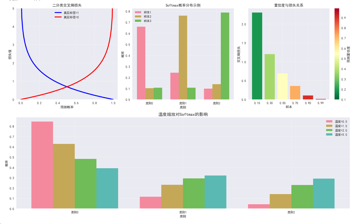
3.1 交叉熵损失 (Cross Entropy Loss)

数学定义：L = -Σ yi * log(ŷi)

特点：

• 多分类任务的标准损失
• 内置Softmax激活
• 概率解释明确

# 交叉熵损失演示
class CrossEntropyDemo:def __init__(self, device):self.device = deviceself.ce_loss = nn.CrossEntropyLoss()def demonstrate(self):# 多分类示例 (3类)batch_size = 32num_classes = 3# 模拟网络输出 (logits)logits = torch.randn(batch_size, num_classes).to(self.device)# 真实标签targets = torch.randint(0, num_classes, (batch_size,)).to(self.device)# 计算损失ce_loss = self.ce_loss(logits, targets)# 手动计算验证probabilities = F.softmax(logits, dim=1)print(f"\n交叉熵损失演示:")print(f"批次大小: {batch_size}, 类别数: {num_classes}")print(f"交叉熵损失: {ce_loss.item():.6f}")print(f"平均概率: {probabilities.mean().item():.4f}")print(f"最大概率: {probabilities.max().item():.4f}")print(f"最小概率: {probabilities.min().item():.4f}")# 展示标签分布unique, counts = torch.unique(targets, return_counts=True)print("标签分布:")for label, count in zip(unique, counts):print(f"  类别 {label.item()}: {count.item()} 样本")return ce_lossce_demo = CrossEntropyDemo(device)
ce_loss = ce_demo.demonstrate()# 可视化交叉熵损失特性
def plot_cross_entropy_analysis():"""分析交叉熵损失的特性"""fig = plt.figure(figsize=(16, 10))gs = GridSpec(2, 3, figure=fig)# 子图1: 二分类交叉熵随概率变化ax1 = fig.add_subplot(gs[0, 0])probs = torch.linspace(0.001, 0.999, 100)# 正类和负类的损失pos_loss = -torch.log(probs)neg_loss = -torch.log(1 - probs)ax1.plot(probs.numpy(), pos_loss.numpy(), 'b-', linewidth=3, label='真实标签=1')ax1.plot(probs.numpy(), neg_loss.numpy(), 'r-', linewidth=3, label='真实标签=0')ax1.set_title('二分类交叉熵损失', fontsize=12, fontweight='bold')ax1.set_xlabel('预测概率')ax1.set_ylabel('损失值')ax1.set_ylim(0, 5)ax1.grid(True, alpha=0.3)ax1.legend()# 子图2: Softmax概率分布ax2 = fig.add_subplot(gs[0, 1])logits = torch.tensor([[2.0, 1.0, 0.1], [0.5, 2.5, 0.8], [1.0, 1.0, 3.0]])probs = F.softmax(logits, dim=1)classes = ['类别0', '类别1', '类别2']x = np.arange(len(classes))width = 0.25for i in range(3):ax2.bar(x + i*width, probs[i].numpy(), width, label=f'样本{i+1}', alpha=0.8)ax2.set_title('Softmax概率分布示例', fontsize=12, fontweight='bold')ax2.set_xlabel('类别')ax2.set_ylabel('概率')ax2.set_xticks(x + width)ax2.set_xticklabels(classes)ax2.legend()ax2.grid(True, alpha=0.3)# 子图3: 置信度对损失的影响ax3 = fig.add_subplot(gs[0, 2])confidences = torch.tensor([0.1, 0.3, 0.5, 0.7, 0.9, 0.99])losses = -torch.log(confidences)colors = plt.cm.RdYlGn_r(confidences.numpy())bars = ax3.bar(range(len(confidences)), losses.numpy(), color=colors)ax3.set_title('置信度与损失关系', fontsize=12, fontweight='bold')ax3.set_xlabel('样本')ax3.set_ylabel('交叉熵损失')ax3.set_xticks(range(len(confidences)))ax3.set_xticklabels([f'{c:.2f}' for c in confidences])ax3.grid(True, alpha=0.3)# 添加颜色条sm = plt.cm.ScalarMappable(cmap=plt.cm.RdYlGn_r, norm=plt.Normalize(vmin=0.1, vmax=0.99))sm.set_array([])cbar = plt.colorbar(sm, ax=ax3)cbar.set_label('预测置信度')# 子图4: 温度缩放效果ax4 = fig.add_subplot(gs[1, :])logits = torch.tensor([2.0, 1.0, 0.5])temperatures = [0.5, 1.0, 2.0, 5.0]x_pos = np.arange(len(logits))width = 0.2for i, temp in enumerate(temperatures):scaled_probs = F.softmax(logits / temp, dim=0)ax4.bar(x_pos + i*width, scaled_probs.numpy(), width, label=f'温度={temp}', alpha=0.8)ax4.set_title('温度缩放对Softmax的影响', fontsize=14, fontweight='bold')ax4.set_xlabel('类别')ax4.set_ylabel('概率')ax4.set_xticks(x_pos + width * 1.5)ax4.set_xticklabels(['类别0', '类别1', '类别2'])ax4.legend()ax4.grid(True, alpha=0.3)plt.tight_layout()plt.show()plot_cross_entropy_analysis()

3.2 二元交叉熵损失 (Binary Cross Entropy Loss)

数学定义：L = -[y*log(ŷ) + (1-y)*log(1-ŷ)]

特点：

• 二分类任务专用
• 需要Sigmoid激活
• 输出概率值

# 二元交叉熵损失演示
class BCELossDemo:def __init__(self, device):self.device = deviceself.bce_loss = nn.BCELoss()self.bce_with_logits = nn.BCEWithLogitsLoss()  # 更数值稳定def demonstrate(self):batch_size = 100# 方式1: 先Sigmoid再BCElogits = torch.randn(batch_size, 1).to(self.device)probabilities = torch.sigmoid(logits)targets = torch.randint(0, 2, (batch_size, 1), dtype=torch.float32).to(self.device)bce_loss = self.bce_loss(probabilities, targets)# 方式2: BCE with Logits (推荐，数值更稳定)bce_logits_loss = self.bce_with_logits(logits, targets)print(f"\n二元交叉熵损失演示:")print(f"BCE Loss: {bce_loss.item():.6f}")print(f"BCE with Logits Loss: {bce_logits_loss.item():.6f}")print(f"预测概率范围: [{probabilities.min().item():.4f}, {probabilities.max().item():.4f}]")# 展示不同置信度对损失的影响print("\n置信度对损失的影响:")test_probs = torch.tensor([0.01, 0.1, 0.5, 0.9, 0.99]).unsqueeze(1).to(self.device)test_targets = torch.ones_like(test_probs)for prob, target in zip(test_probs, test_targets):loss = self.bce_loss(prob, target)print(f"预测概率: {prob.item():.2f}, 损失: {loss.item():.4f}")return bce_logits_lossbce_demo = BCELossDemo(device)
bce_loss = bce_demo.demonstrate()

二元交叉熵损失演示:
BCE Loss: 0.809278
BCE with Logits Loss: 0.809278
预测概率范围: [0.1330, 0.9427]

置信度对损失的影响:
预测概率: 0.01, 损失: 4.6052
预测概率: 0.10, 损失: 2.3026
预测概率: 0.50, 损失: 0.6931
预测概率: 0.90, 损失: 0.1054
预测概率: 0.99, 损失: 0.0101

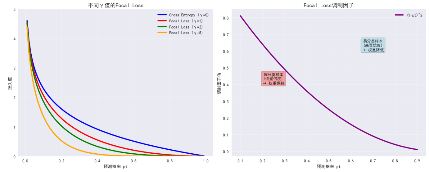
3.3 Focal Loss

数学定义：FL = -α(1-pt)^γ * log(pt)

特点：

• 解决类别不平衡问题
• 关注困难样本
• 降低易分类样本权重

# Focal Loss实现
class FocalLoss(nn.Module):def __init__(self, alpha=1.0, gamma=2.0, reduction='mean'):super(FocalLoss, self).__init__()self.alpha = alphaself.gamma = gammaself.reduction = reductiondef forward(self, inputs, targets):# 计算交叉熵ce_loss = F.cross_entropy(inputs, targets, reduction='none')# 计算概率pt = torch.exp(-ce_loss)# 计算Focal Lossfocal_loss = self.alpha * (1 - pt) ** self.gamma * ce_lossif self.reduction == 'mean':return focal_loss.mean()elif self.reduction == 'sum':return focal_loss.sum()else:return focal_loss# Focal Loss演示
class FocalLossDemo:def __init__(self, device):self.device = deviceself.focal_loss = FocalLoss(alpha=1.0, gamma=2.0).to(device)self.ce_loss = nn.CrossEntropyLoss()def demonstrate(self):# 创建不平衡数据集batch_size = 1000num_classes = 3logits = torch.randn(batch_size, num_classes).to(self.device)# 创建不平衡标签 (类别0占70%, 类别1占25%, 类别2占5%)targets = torch.cat([torch.zeros(700, dtype=torch.long),torch.ones(250, dtype=torch.long),torch.full((50,), 2, dtype=torch.long)]).to(self.device)# 随机打乱idx = torch.randperm(batch_size)targets = targets[idx]# 比较Focal Loss和交叉熵损失focal_loss_val = self.focal_loss(logits, targets)ce_loss_val = self.ce_loss(logits, targets)print(f"\nFocal Loss vs Cross Entropy (不平衡数据集):")print(f"数据分布: 类别0: 70%, 类别1: 25%, 类别2: 5%")print(f"Focal Loss: {focal_loss_val.item():.6f}")print(f"Cross Entropy Loss: {ce_loss_val.item():.6f}")# 分析各类别的平均损失with torch.no_grad():probabilities = F.softmax(logits, dim=1)for class_id in range(num_classes):class_mask = targets == class_idif class_mask.sum() > 0:class_probs = probabilities[class_mask, class_id]avg_prob = class_probs.mean()print(f"类别 {class_id} 平均预测概率: {avg_prob.item():.4f}")return focal_loss_valfocal_demo = FocalLossDemo(device)
focal_loss = focal_demo.demonstrate()# 可视化Focal Loss特性
def plot_focal_loss_analysis():"""分析Focal Loss的特性和效果"""fig, ((ax1, ax2), (ax3, ax4)) = plt.subplots(2, 2, figsize=(15, 12))# 子图1: 不同γ值的Focal Losspt = torch.linspace(0.01, 0.99, 100)gammas = [0, 1, 2, 5]colors = ['blue', 'red', 'green', 'orange']for gamma, color in zip(gammas, colors):if gamma == 0:focal_loss = -torch.log(pt)  # 标准交叉熵label = 'Cross Entropy (γ=0)'else:focal_loss = -(1 - pt)**gamma * torch.log(pt)label = f'Focal Loss (γ={gamma})'ax1.plot(pt.numpy(), focal_loss.numpy(), color=color, linewidth=3, label=label)ax1.set_title('不同γ值的Focal Loss', fontsize=14, fontweight='bold')ax1.set_xlabel('预测概率 pt')ax1.set_ylabel('损失值')ax1.set_ylim(0, 5)ax1.grid(True, alpha=0.3)ax1.legend()# 子图2: 调制因子的影响pt_range = torch.linspace(0.1, 0.9, 50)gamma = 2modulating_factor = (1 - pt_range)**gammaax2.plot(pt_range.numpy(), modulating_factor.numpy(), 'purple', linewidth=3, label=f'(1-pt)^{gamma}')ax2.set_title('Focal Loss调制因子', fontsize=14, fontweight='bold')ax2.set_xlabel('预测概率 pt')ax2.set_ylabel('调制因子值')ax2.grid(True, alpha=0.3)ax2.legend()# 添加说明文本ax2.text(0.7, 0.6, '易分类样本\n(高置信度)\n→ 权重降低', bbox=dict(boxstyle="round,pad=0.3", facecolor="lightblue", alpha=0.7),fontsize=10, ha='center')ax2.text(0.25, 0.4, '难分类样本\n(低置信度)\n→ 权重保持', bbox=dict(boxstyle="round,pad=0.3", facecolor="lightcoral", alpha=0.7),fontsize=10, ha='center')# 子图3: 类别不平衡数据模拟# 模拟不平衡数据集的损失分布np.random.seed(42)n_majority = 900n_minority = 100# 模拟预测概率（多数类通常预测更准确）majority_probs = np.random.beta(7, 2, n_majority)  # 偏向高概率minority_probs = np.random.beta(2, 3, n_minority)  # 偏向低概率ax3.hist(majority_probs, bins=30, alpha=0.7, label=f'多数类 ({n_majority}样本)', color='blue', density=True)ax3.hist(minority_probs, bins=30, alpha=0.7, label=f'少数类 ({n_minority}样本)', color='red', density=True)ax3.set_title('不平衡数据的预测概率分布', fontsize=14, fontweight='bold')ax3.set_xlabel('预测概率')ax3.set_ylabel('密度')ax3.legend()ax3.grid(True, alpha=0.3)# 子图4: Focal Loss vs Cross Entropy损失对比ce_majority = -np.log(np.clip(majority_probs, 1e-7, 1-1e-7))ce_minority = -np.log(np.clip(minority_probs, 1e-7, 1-1e-7))focal_majority = -(1 - majority_probs)**2 * np.log(np.clip(majority_probs, 1e-7, 1-1e-7))focal_minority = -(1 - minority_probs)**2 * np.log(np.clip(minority_probs, 1e-7, 1-1e-7))loss_comparison = {'Cross Entropy': [ce_majority.mean(), ce_minority.mean()],'Focal Loss': [focal_majority.mean(), focal_minority.mean()]}x = np.arange(2)width = 0.35ce_bars = ax4.bar(x - width/2, loss_comparison['Cross Entropy'], width, label='Cross Entropy', alpha=0.8, color='skyblue')focal_bars = ax4.bar(x + width/2, loss_comparison['Focal Loss'], width, label='Focal Loss', alpha=0.8, color='lightcoral')ax4.set_title('平均损失对比', fontsize=14, fontweight='bold')ax4.set_ylabel('平均损失值')ax4.set_xticks(x)ax4.set_xticklabels(['多数类', '少数类'])ax4.legend()ax4.grid(True, alpha=0.3)# 添加数值标签for bar in ce_bars:height = bar.get_height()ax4.text(bar.get_x() + bar.get_width()/2., height + 0.01,f'{height:.3f}', ha='center', va='bottom')for bar in focal_bars:height = bar.get_height()ax4.text(bar.get_x() + bar.get_width()/2., height + 0.01,f'{height:.3f}', ha='center', va='bottom')plt.tight_layout()plt.show()plot_focal_loss_analysis()

4. 自定义损失函数

# 自定义损失函数示例: Dice Loss (用于分割任务)
class DiceLoss(nn.Module):def __init__(self, smooth=1e-5):super(DiceLoss, self).__init__()self.smooth = smoothdef forward(self, predictions, targets):# 展平预测和目标predictions = predictions.view(-1)targets = targets.view(-1)# 计算交集和并集intersection = (predictions * targets).sum()dice_coeff = (2. * intersection + self.smooth) / (predictions.sum() + targets.sum() + self.smooth)return 1 - dice_coeff# Dice Loss演示
class DiceLossDemo:def __init__(self, device):self.device = deviceself.dice_loss = DiceLoss().to(device)def demonstrate(self):# 模拟分割任务batch_size = 4height, width = 64, 64# 创建模拟的分割图targets = torch.randint(0, 2, (batch_size, 1, height, width), dtype=torch.float32).to(self.device)# 创建带噪声的预测predictions = targets + 0.1 * torch.randn_like(targets)predictions = torch.sigmoid(predictions)  # 转换为概率# 计算Dice Lossdice_loss_val = self.dice_loss(predictions, targets)print(f"\nDice Loss演示 (分割任务):")print(f"图像大小: {height}x{width}")print(f"批次大小: {batch_size}")print(f"Dice Loss: {dice_loss_val.item():.6f}")print(f"平均预测概率: {predictions.mean().item():.4f}")print(f"目标像素比例: {targets.mean().item():.4f}")return dice_loss_valdice_demo = DiceLossDemo(device)
dice_loss = dice_demo.demonstrate()

Dice Loss演示 (分割任务):
图像大小: 64x64
批次大小: 4
Dice Loss: 0.345719
平均预测概率: 0.6149
目标像素比例: 0.4985

实战案例

完整的神经网络训练示例

# 完整的分类网络示例
class CompleteClassificationNet(nn.Module):def __init__(self, input_size, hidden_size, num_classes, activation='relu', dropout_rate=0.5):super(CompleteClassificationNet, self).__init__()self.fc1 = nn.Linear(input_size, hidden_size)self.fc2 = nn.Linear(hidden_size, hidden_size)self.fc3 = nn.Linear(hidden_size, num_classes)self.dropout = nn.Dropout(dropout_rate)# 选择激活函数if activation == 'relu':self.activation = nn.ReLU()elif activation == 'tanh':self.activation = nn.Tanh()elif activation == 'gelu':self.activation = nn.GELU()else:self.activation = nn.ReLU()  # 默认def forward(self, x):x = self.activation(self.fc1(x))x = self.dropout(x)x = self.activation(self.fc2(x))x = self.dropout(x)x = self.fc3(x)  # 不加激活，让损失函数处理return x# 训练函数
def train_model(model, train_loader, criterion, optimizer, device, num_epochs=10):model.train()train_losses = []for epoch in range(num_epochs):epoch_loss = 0.0correct = 0total = 0for batch_idx, (data, targets) in enumerate(train_loader):data, targets = data.to(device), targets.to(device)# 前向传播outputs = model(data)loss = criterion(outputs, targets)# 反向传播optimizer.zero_grad()loss.backward()optimizer.step()# 统计epoch_loss += loss.item()_, predicted = torch.max(outputs.data, 1)total += targets.size(0)correct += (predicted == targets).sum().item()avg_loss = epoch_loss / len(train_loader)accuracy = 100 * correct / totaltrain_losses.append(avg_loss)if epoch % 2 == 0:print(f'Epoch [{epoch+1}/{num_epochs}], Loss: {avg_loss:.6f}, Accuracy: {accuracy:.2f}%')return train_losses# 创建示例数据集
def create_sample_dataset(num_samples=1000, input_size=20, num_classes=3):# 生成随机数据X = torch.randn(num_samples, input_size)# 创建有意义的标签y = ((X[:, :3].sum(dim=1) + X[:, 3:6].sum(dim=1)) > 0).long()y = y % num_classes  # 确保在类别范围内return X, y# 主训练演示
def main_training_demo():print("\n=== 完整训练演示 ===")# 参数设置input_size = 20hidden_size = 128num_classes = 3batch_size = 32learning_rate = 0.001num_epochs = 20# 创建数据X, y = create_sample_dataset(1000, input_size, num_classes)dataset = torch.utils.data.TensorDataset(X, y)train_loader = torch.utils.data.DataLoader(dataset, batch_size=batch_size, shuffle=True)# 比较不同激活函数的性能activations = ['relu', 'tanh', 'gelu']results = {}for activation in activations:print(f"\n--- 使用 {activation.upper()} 激活函数 ---")# 创建模型model = CompleteClassificationNet(input_size, hidden_size, num_classes, activation).to(device)# 损失函数和优化器criterion = nn.CrossEntropyLoss()optimizer = torch.optim.Adam(model.parameters(), lr=learning_rate)# 训练模型train_losses = train_model(model, train_loader, criterion, optimizer, device, num_epochs)results[activation] = {'final_loss': train_losses[-1],'model': model,'losses': train_losses}print(f"最终损失: {train_losses[-1]:.6f}")# 结果比较print("\n=== 激活函数性能比较 ===")for activation, result in results.items():print(f"{activation.upper()}: 最终损失 = {result['final_loss']:.6f}")return results# 执行训练演示
training_results = main_training_demo()

=== 完整训练演示 ===

— 使用 RELU 激活函数 —
Epoch [1/20], Loss: 0.826066, Accuracy: 59.30%
Epoch [3/20], Loss: 0.401554, Accuracy: 83.20%
Epoch [5/20], Loss: 0.265561, Accuracy: 88.00%
Epoch [7/20], Loss: 0.165232, Accuracy: 93.60%
Epoch [9/20], Loss: 0.160084, Accuracy: 93.40%
Epoch [11/20], Loss: 0.157044, Accuracy: 93.00%
Epoch [13/20], Loss: 0.130174, Accuracy: 94.30%
Epoch [15/20], Loss: 0.133823, Accuracy: 94.20%
Epoch [17/20], Loss: 0.091265, Accuracy: 96.60%
Epoch [19/20], Loss: 0.100133, Accuracy: 95.60%
最终损失: 0.096137

— 使用 TANH 激活函数 —
Epoch [1/20], Loss: 0.826223, Accuracy: 64.50%
Epoch [3/20], Loss: 0.275804, Accuracy: 90.50%
Epoch [5/20], Loss: 0.185776, Accuracy: 92.60%
Epoch [7/20], Loss: 0.161310, Accuracy: 93.40%
Epoch [9/20], Loss: 0.139488, Accuracy: 93.40%
Epoch [11/20], Loss: 0.126005, Accuracy: 93.70%
Epoch [13/20], Loss: 0.103266, Accuracy: 95.30%
Epoch [15/20], Loss: 0.108249, Accuracy: 95.90%
Epoch [17/20], Loss: 0.112322, Accuracy: 95.20%
Epoch [19/20], Loss: 0.109068, Accuracy: 96.20%
最终损失: 0.091335

— 使用 GELU 激活函数 —
Epoch [1/20], Loss: 0.907230, Accuracy: 61.00%
Epoch [3/20], Loss: 0.353793, Accuracy: 86.00%
Epoch [5/20], Loss: 0.216205, Accuracy: 91.00%
Epoch [7/20], Loss: 0.171754, Accuracy: 92.20%
Epoch [9/20], Loss: 0.155852, Accuracy: 92.90%
Epoch [11/20], Loss: 0.134879, Accuracy: 95.30%
Epoch [13/20], Loss: 0.124601, Accuracy: 95.00%
Epoch [15/20], Loss: 0.092257, Accuracy: 96.10%
Epoch [17/20], Loss: 0.082220, Accuracy: 96.70%
Epoch [19/20], Loss: 0.073818, Accuracy: 97.10%
最终损失: 0.084081

=== 激活函数性能比较 ===
RELU: 最终损失 = 0.096137
TANH: 最终损失 = 0.091335
GELU: 最终损失 = 0.084081

性能优化技巧

1. 数值稳定性

# 数值稳定性技巧
def numerical_stability_demo():print("\n=== 数值稳定性演示 ===")# 极端值测试extreme_logits = torch.tensor([[-100., -50., 100.]], device=device)targets = torch.tensor([2], device=device)# 不稳定的实现def unstable_cross_entropy(logits, targets):# 手动实现Softmax + CrossEntropy (数值不稳定)exp_logits = torch.exp(logits)softmax_probs = exp_logits / exp_logits.sum(dim=1, keepdim=True)log_probs = torch.log(softmax_probs)return -log_probs.gather(1, targets.unsqueeze(1)).mean()# 稳定的实现def stable_cross_entropy(logits, targets):return F.cross_entropy(logits, targets)print("极端logits测试:")print(f"Logits: {extreme_logits}")try:unstable_loss = unstable_cross_entropy(extreme_logits, targets)print(f"不稳定实现损失: {unstable_loss.item():.6f}")except Exception as e:print(f"不稳定实现失败: {e}")stable_loss = stable_cross_entropy(extreme_logits, targets)print(f"稳定实现损失: {stable_loss.item():.6f}")# LogSumExp技巧演示print("\n=== LogSumExp数值稳定技巧 ===")def log_sum_exp_unstable(x):return torch.log(torch.sum(torch.exp(x), dim=1))def log_sum_exp_stable(x):max_x = torch.max(x, dim=1, keepdim=True)[0]return max_x.squeeze(1) + torch.log(torch.sum(torch.exp(x - max_x), dim=1))test_logits = torch.tensor([[100., 101., 102.]], device=device)try:unstable_result = log_sum_exp_unstable(test_logits)print(f"不稳定LogSumExp: {unstable_result.item():.6f}")except Exception as e:print(f"不稳定LogSumExp失败: {e}")stable_result = log_sum_exp_stable(test_logits)print(f"稳定LogSumExp: {stable_result.item():.6f}")pytorch_result = torch.logsumexp(test_logits, dim=1)print(f"PyTorch LogSumExp: {pytorch_result.item():.6f}")numerical_stability_demo()

=== 数值稳定性演示 ===
极端logits测试:
Logits: tensor([[-100., -50., 100.]], device=‘cuda:0’)
不稳定实现损失: nan
稳定实现损失: 0.000000

=== LogSumExp数值稳定技巧 ===
不稳定LogSumExp: inf
稳定LogSumExp: 102.407608
PyTorch LogSumExp: 102.407608

2. 梯度流分析

# 梯度流分析
class GradientFlowAnalyzer:def __init__(self, device):self.device = devicedef analyze_activation_gradients(self):print("\n=== 激活函数梯度流分析 ===")# 创建深层网络测试梯度流class DeepNet(nn.Module):def __init__(self, activation_func, num_layers=10):super(DeepNet, self).__init__()layers = []for i in range(num_layers):layers.append(nn.Linear(128, 128))if activation_func == 'relu':layers.append(nn.ReLU())elif activation_func == 'sigmoid':layers.append(nn.Sigmoid())elif activation_func == 'tanh':layers.append(nn.Tanh())elif activation_func == 'gelu':layers.append(nn.GELU())layers.append(nn.Linear(128, 1))self.network = nn.Sequential(*layers)def forward(self, x):return self.network(x)activations = ['relu', 'sigmoid', 'tanh', 'gelu']gradient_stats = {}for activation in activations:model = DeepNet(activation).to(self.device)x = torch.randn(32, 128, requires_grad=True).to(self.device)# 前向传播output = model(x).sum()# 反向传播output.backward()# 收集梯度统计gradients = []for name, param in model.named_parameters():if param.grad is not None and 'weight' in name:gradients.append(param.grad.abs().mean().item())gradient_stats[activation] = {'mean_grad': np.mean(gradients),'min_grad': np.min(gradients),'max_grad': np.max(gradients),'std_grad': np.std(gradients)}print(f"\n{activation.upper()} 激活函数梯度统计:")print(f"  平均梯度: {gradient_stats[activation]['mean_grad']:.6f}")print(f"  最小梯度: {gradient_stats[activation]['min_grad']:.6f}")print(f"  最大梯度: {gradient_stats[activation]['max_grad']:.6f}")print(f"  梯度标准差: {gradient_stats[activation]['std_grad']:.6f}")return gradient_statsdef analyze_loss_gradients(self):print("\n=== 损失函数梯度分析 ===")# 创建测试数据x = torch.randn(100, 10, requires_grad=True).to(self.device)true_targets = torch.randn(100, 1).to(self.device)class_targets = torch.randint(0, 3, (100,)).to(self.device)loss_functions = {'MSE': nn.MSELoss(),'MAE': nn.L1Loss(),'Smooth_L1': nn.SmoothL1Loss(),'CrossEntropy': nn.CrossEntropyLoss()}# 简单网络model = nn.Sequential(nn.Linear(10, 20),nn.ReLU(),nn.Linear(20, 3)).to(self.device)for loss_name, loss_func in loss_functions.items():model.zero_grad()outputs = model(x)if loss_name == 'CrossEntropy':loss = loss_func(outputs, class_targets)else:# 对于回归损失，使用输出的第一列loss = loss_func(outputs[:, 0:1], true_targets)loss.backward()# 计算梯度范数total_norm = 0for param in model.parameters():if param.grad is not None:total_norm += param.grad.data.norm(2).item() ** 2total_norm = total_norm ** 0.5print(f"{loss_name} 损失梯度范数: {total_norm:.6f}")gradient_analyzer = GradientFlowAnalyzer(device)
grad_stats = gradient_analyzer.analyze_activation_gradients()
gradient_analyzer.analyze_loss_gradients()

=== 激活函数梯度流分析 ===

RELU 激活函数梯度统计:
平均梯度: 0.058187
最小梯度: 0.000078
最大梯度: 0.614190
梯度标准差: 0.175872

SIGMOID 激活函数梯度统计:
平均梯度: 1.465491
最小梯度: 0.000000
最大梯度: 15.923494
梯度标准差: 4.572277

TANH 激活函数梯度统计:
平均梯度: 0.168461
最小梯度: 0.000839
最大梯度: 1.688113
梯度标准差: 0.481087

GELU 激活函数梯度统计:
平均梯度: 0.069552
最小梯度: 0.000002
最大梯度: 0.742825
梯度标准差: 0.212954

=== 损失函数梯度分析 ===
MSE 损失梯度范数: 0.872801
MAE 损失梯度范数: 0.469781
Smooth_L1 损失梯度范数: 0.291672
CrossEntropy 损失梯度范数: 0.379675

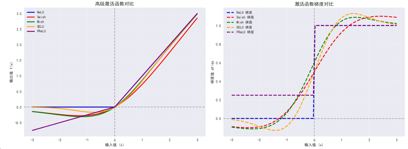
3. 高级激活函数

import torch
import torch.nn as nn
import torch.nn.functional as F
import matplotlib.pyplot as plt
import numpy as np# 设置中文字体支持
plt.rcParams['font.sans-serif'] = ['SimHei', 'DejaVu Sans']
plt.rcParams['axes.unicode_minus'] = False# 检查设备
device = torch.device('cuda' if torch.cuda.is_available() else 'cpu')
print(f"使用设备: {device}")# 高级激活函数实现
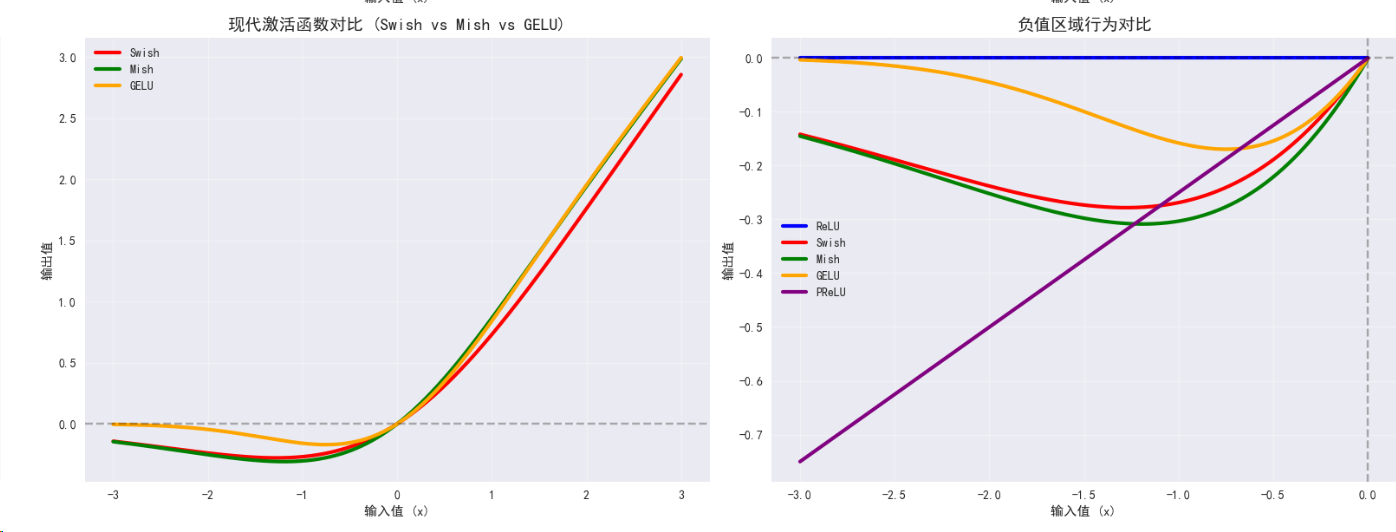
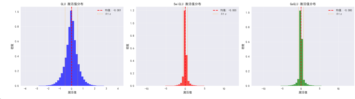
class AdvancedActivations:def __init__(self, device):self.device = devicedef swish_mish_comparison(self):print("\n=== Swish与Mish激活函数比较 ===")# Swish激活函数class Swish(nn.Module):def forward(self, x):return x * torch.sigmoid(x)# Mish激活函数class Mish(nn.Module):def forward(self, x):return x * torch.tanh(F.softplus(x))# 自适应激活函数 (PReLU)class AdaptivePReLU(nn.Module):def __init__(self, num_parameters=1, init=0.25):super(AdaptivePReLU, self).__init__()self.num_parameters = num_parametersself.weight = nn.Parameter(torch.Tensor(num_parameters).fill_(init))def forward(self, x):return F.prelu(x, self.weight)# 测试输入x = torch.linspace(-3, 3, 1000).to(self.device)activations = {'ReLU': nn.ReLU(),'Swish': Swish(),'Mish': Mish(),'GELU': nn.GELU(),'PReLU': AdaptivePReLU()}results = {}# 计算激活函数输出for name, activation in activations.items():activation = activation.to(self.device)with torch.no_grad():y = activation(x)results[name] = y.cpu()print(f"{name} 输出范围: [{y.min().item():.4f}, {y.max().item():.4f}]")# 修复的梯度计算 - 为每个激活函数单独创建输入张量print("\n梯度特性比较:")gradients = {}for name, activation in activations.items():# 为每个激活函数创建新的输入张量x_grad = torch.linspace(-3, 3, 100, requires_grad=True, device=self.device)activation = activation.to(self.device)# 前向传播和反向传播y = activation(x_grad).sum()y.backward()# 计算梯度统计if x_grad.grad is not None:grad_mean = x_grad.grad.abs().mean().item()grad_std = x_grad.grad.std().item()gradients[name] = x_grad.grad.clone().detach()print(f"{name} - 平均梯度: {grad_mean:.4f}, 梯度标准差: {grad_std:.4f}")else:print(f"{name} - 梯度计算失败")# 可视化比较self.plot_advanced_activations(results, gradients)return resultsdef plot_advanced_activations(self, results, gradients):"""绘制高级激活函数对比图"""fig, ((ax1, ax2), (ax3, ax4)) = plt.subplots(2, 2, figsize=(16, 12))x_range = torch.linspace(-3, 3, 1000)x_grad_range = torch.linspace(-3, 3, 100)# 子图1: 所有激活函数对比colors = ['blue', 'red', 'green', 'orange', 'purple']for i, (name, y) in enumerate(results.items()):ax1.plot(x_range, y, linewidth=2.5, label=name, color=colors[i])ax1.set_title('高级激活函数对比', fontsize=14, fontweight='bold')ax1.set_xlabel('输入值 (x)')ax1.set_ylabel('输出值 f(x)')ax1.grid(True, alpha=0.3)ax1.legend()ax1.axhline(y=0, color='k', linestyle='--', alpha=0.3)ax1.axvline(x=0, color='k', linestyle='--', alpha=0.3)# 子图2: 梯度对比for i, (name, grad) in enumerate(gradients.items()):if grad is not None:ax2.plot(x_grad_range, grad.cpu(), linewidth=2.5, label=f"{name} 梯度", linestyle='--', color=colors[i])ax2.set_title('激活函数梯度对比', fontsize=14, fontweight='bold')ax2.set_xlabel('输入值 (x)')ax2.set_ylabel('梯度值 df/dx')ax2.grid(True, alpha=0.3)ax2.legend()ax2.axhline(y=0, color='k', linestyle='--', alpha=0.3)ax2.axvline(x=0, color='k', linestyle='--', alpha=0.3)# 子图3: Swish vs Mish vs GELU 特写modern_activations = ['Swish', 'Mish', 'GELU']modern_colors = ['red', 'green', 'orange']for i, name in enumerate(modern_activations):if name in results:ax3.plot(x_range, results[name], linewidth=3, label=name, color=modern_colors[i])ax3.set_title('现代激活函数对比 (Swish vs Mish vs GELU)', fontsize=14, fontweight='bold')ax3.set_xlabel('输入值 (x)')ax3.set_ylabel('输出值')ax3.grid(True, alpha=0.3)ax3.legend()ax3.axhline(y=0, color='k', linestyle='--', alpha=0.3)# 子图4: 负值区域的行为对比x_neg = torch.linspace(-3, 0, 500)for i, (name, y) in enumerate(results.items()):y_neg = y[:500]  # 取负值部分ax4.plot(x_neg, y_neg, linewidth=3, label=name, color=colors[i])ax4.set_title('负值区域行为对比', fontsize=14, fontweight='bold')ax4.set_xlabel('输入值 (x)')ax4.set_ylabel('输出值')ax4.grid(True, alpha=0.3)ax4.legend()ax4.axhline(y=0, color='k', linestyle='--', alpha=0.3)ax4.axvline(x=0, color='k', linestyle='--', alpha=0.3)plt.tight_layout()plt.show()def attention_activations(self):print("\n=== 注意力机制中的激活函数 ===")# GLU (Gated Linear Unit)class GLU(nn.Module):def __init__(self, dim=-1):super(GLU, self).__init__()self.dim = dimdef forward(self, x):a, b = x.chunk(2, dim=self.dim)return a * torch.sigmoid(b)# Swish-GLU (SwiGLU)class SwiGLU(nn.Module):def __init__(self, dim=-1):super(SwiGLU, self).__init__()self.dim = dimdef forward(self, x):a, b = x.chunk(2, dim=self.dim)return a * (b * torch.sigmoid(b))  # Swish(b) = b * sigmoid(b)# GeGLU (GELU + GLU)class GeGLU(nn.Module):def __init__(self, dim=-1):super(GeGLU, self).__init__()self.dim = dimdef forward(self, x):a, b = x.chunk(2, dim=self.dim)return a * F.gelu(b)# 测试数据batch_size, seq_len, hidden_dim = 32, 128, 512x = torch.randn(batch_size, seq_len, hidden_dim * 2).to(self.device)  # *2 for GLUglu_variants = {'GLU': GLU(),'SwiGLU': SwiGLU(),'GeGLU': GeGLU()}print(f"输入形状: {x.shape}")outputs = {}for name, glu_layer in glu_variants.items():glu_layer = glu_layer.to(self.device)with torch.no_grad():output = glu_layer(x)outputs[name] = outputprint(f"{name}输出形状: {output.shape}")print(f"{name}输出范围: [{output.min().item():.4f}, {output.max().item():.4f}]")print(f"{name}输出均值: {output.mean().item():.4f}, 标准差: {output.std().item():.4f}")# 分析不同GLU变体的激活模式self.analyze_glu_patterns(outputs)return outputsdef analyze_glu_patterns(self, outputs):"""分析GLU变体的激活模式"""print("\n--- GLU变体激活模式分析 ---")fig, axes = plt.subplots(1, 3, figsize=(18, 5))for i, (name, output) in enumerate(outputs.items()):# 计算激活值的分布output_flat = output.cpu().flatten()# 绘制激活值分布直方图axes[i].hist(output_flat, bins=50, alpha=0.7, density=True, color=['blue', 'red', 'green'][i])axes[i].set_title(f'{name} 激活值分布', fontsize=12, fontweight='bold')axes[i].set_xlabel('激活值')axes[i].set_ylabel('密度')axes[i].grid(True, alpha=0.3)# 添加统计信息mean_val = output_flat.mean().item()std_val = output_flat.std().item()axes[i].axvline(mean_val, color='red', linestyle='--', linewidth=2, label=f'均值: {mean_val:.3f}')axes[i].axvline(mean_val + std_val, color='orange', linestyle=':', alpha=0.7, label=f'±1σ')axes[i].axvline(mean_val - std_val, color='orange', linestyle=':', alpha=0.7)axes[i].legend()# 计算激活稀疏性 (接近0的值的比例)sparse_ratio = (output_flat.abs() < 0.1).float().mean().item()print(f"{name} 稀疏性 (|x|<0.1): {sparse_ratio:.3f}")plt.tight_layout()plt.show()def activation_function_benchmark(self):"""激活函数性能基准测试"""print("\n=== 激活函数性能基准测试 ===")# 定义所有激活函数class Swish(nn.Module):def forward(self, x):return x * torch.sigmoid(x)class Mish(nn.Module):def forward(self, x):return x * torch.tanh(F.softplus(x))activations = {'ReLU': nn.ReLU(),'GELU': nn.GELU(),'Swish': Swish(),'Mish': Mish(),'Sigmoid': nn.Sigmoid(),'Tanh': nn.Tanh()}# 测试数据test_sizes = [1000, 10000, 100000]import timeresults = {}for size in test_sizes:print(f"\n测试数据大小: {size}")x = torch.randn(size).to(self.device)for name, activation in activations.items():activation = activation.to(self.device)# 预热with torch.no_grad():_ = activation(x)# 计时测试torch.cuda.synchronize() if self.device.type == 'cuda' else Nonestart_time = time.time()with torch.no_grad():for _ in range(100):  # 重复100次_ = activation(x)torch.cuda.synchronize() if self.device.type == 'cuda' else Noneend_time = time.time()avg_time = (end_time - start_time) / 100 * 1000  # 转换为毫秒if name not in results:results[name] = []results[name].append(avg_time)print(f"{name}: {avg_time:.4f} ms")# 绘制性能对比图self.plot_performance_benchmark(results, test_sizes)return resultsdef plot_performance_benchmark(self, results, test_sizes):"""绘制性能基准测试结果"""plt.figure(figsize=(12, 8))colors = ['blue', 'red', 'green', 'orange', 'purple', 'brown']for i, (name, times) in enumerate(results.items()):plt.plot(test_sizes, times, marker='o', linewidth=2.5, label=name, color=colors[i % len(colors)])plt.title('激活函数性能基准测试', fontsize=14, fontweight='bold')plt.xlabel('输入数据大小')plt.ylabel('平均执行时间 (毫秒)')plt.legend()plt.grid(True, alpha=0.3)plt.xscale('log')plt.yscale('log')plt.tight_layout()plt.show()# 使用示例
def run_advanced_activation_analysis():"""运行完整的高级激活函数分析"""advanced_activations = AdvancedActivations(device)# 1. Swish与Mish比较swish_mish_results = advanced_activations.swish_mish_comparison()# 2. 注意力机制激活函数attention_results = advanced_activations.attention_activations()# 3. 性能基准测试benchmark_results = advanced_activations.activation_function_benchmark()# 4. 激活函数选择建议print("\n" + "="*60)print("激活函数选择建议")print("="*60)print("\n🎯 根据应用场景选择激活函数:")print("\n1. 传统深度学习任务:")print("   - ReLU: 简单有效，适合大多数情况")print("   - GELU: 性能更好，计算成本稍高")print("\n2. Transformer和注意力模型:")print("   - GELU: 标准选择，性能优异")print("   - Swish: 替代选择，平滑性好")print("   - SwiGLU: 用于FFN层，效果出色")print("\n3. 计算资源受限:")print("   - ReLU: 最快的选择")print("   - 避免使用Mish (计算复杂)")print("\n4. 需要平滑函数:")print("   - GELU: 平衡性能和平滑性")print("   - Swish: 自门控特性")print("   - Mish: 更平滑但计算成本高")return {'swish_mish': swish_mish_results,'attention': attention_results,'benchmark': benchmark_results}# 执行分析
if __name__ == "__main__":results = run_advanced_activation_analysis()

=== Swish与Mish激活函数比较 ===
ReLU 输出范围: [0.0000, 3.0000]
Swish 输出范围: [-0.2785, 2.8577]
Mish 输出范围: [-0.3088, 2.9865]
GELU 输出范围: [-0.1700, 2.9960]
PReLU 输出范围: [-0.7500, 3.0000]

梯度特性比较:
ReLU - 平均梯度: 0.5000, 梯度标准差: 0.5025
Swish - 平均梯度: 0.5458, 梯度标准差: 0.4894
Mish - 平均梯度: 0.5762, 梯度标准差: 0.5058
GELU - 平均梯度: 0.5548, 梯度标准差: 0.5242
PReLU - 平均梯度: 0.6250, 梯度标准差: 0.3769

=== 注意力机制中的激活函数 ===
输入形状: torch.Size([32, 128, 1024])
GLU输出形状: torch.Size([32, 128, 512])
GLU输出范围: [-3.9709, 4.0830]
GLU输出均值: -0.0006, 标准差: 0.5416
SwiGLU输出形状: torch.Size([32, 128, 512])
SwiGLU输出范围: [-11.4914, 12.6636]
SwiGLU输出均值: -0.0003, 标准差: 0.5971
GeGLU输出形状: torch.Size([32, 128, 512])
GeGLU输出范围: [-11.9343, 12.9919]
GeGLU输出均值: -0.0004, 标准差: 0.6527

— GLU变体激活模式分析 —
GLU 稀疏性 (|x|<0.1): 0.202
SwiGLU 稀疏性 (|x|<0.1): 0.383
GeGLU 稀疏性 (|x|<0.1): 0.462

=== 激活函数性能基准测试 ===

测试数据大小: 1000
ReLU: 0.0200 ms
GELU: 0.0100 ms
Swish: 0.0200 ms
Mish: 0.0400 ms
Sigmoid: 0.0100 ms
Tanh: 0.0200 ms

测试数据大小: 10000
ReLU: 0.0100 ms
GELU: 0.0100 ms
Swish: 0.0300 ms
Mish: 0.0400 ms
Sigmoid: 0.0300 ms
Tanh: 0.0800 ms

测试数据大小: 100000
ReLU: 0.0800 ms
GELU: 0.0300 ms
Swish: 0.0400 ms
Mish: 0.3100 ms
Sigmoid: 0.0300 ms
Tanh: 0.0200 ms

. 传统深度学习任务:

• ReLU: 简单有效，适合大多数情况
• GELU: 性能更好，计算成本稍高

2. Transformer和注意力模型:

   • GELU: 标准选择，性能优异
   • Swish: 替代选择，平滑性好
   • SwiGLU: 用于FFN层，效果出色

3. 计算资源受限:

   • ReLU: 最快的选择
   • 避免使用Mish (计算复杂)

4. 需要平滑函数:

   • GELU: 平衡性能和平滑性
   • Swish: 自门控特性
   • Mish: 更平滑但计算成本高

4. 损失函数高级应用

# 高级损失函数应用
class AdvancedLossFunctions:def __init__(self, device):self.device = devicedef contrastive_loss_demo(self):print("\n=== 对比学习损失函数 ===")# 对比损失 (Contrastive Loss)class ContrastiveLoss(nn.Module):def __init__(self, margin=1.0):super(ContrastiveLoss, self).__init__()self.margin = margindef forward(self, output1, output2, label):# label: 1 for similar, 0 for dissimilareuclidean_distance = F.pairwise_distance(output1, output2)loss_contrastive = torch.mean((label) * torch.pow(euclidean_distance, 2) +(1 - label) * torch.pow(torch.clamp(self.margin - euclidean_distance, min=0.0), 2))return loss_contrastive# Triplet Lossclass TripletLoss(nn.Module):def __init__(self, margin=1.0):super(TripletLoss, self).__init__()self.margin = margindef forward(self, anchor, positive, negative):distance_positive = F.pairwise_distance(anchor, positive)distance_negative = F.pairwise_distance(anchor, negative)losses = torch.relu(distance_positive - distance_negative + self.margin)return losses.mean()# 生成示例数据batch_size = 64embedding_dim = 128# 对比损失测试output1 = torch.randn(batch_size, embedding_dim).to(self.device)output2 = torch.randn(batch_size, embedding_dim).to(self.device)labels = torch.randint(0, 2, (batch_size,), dtype=torch.float).to(self.device)contrastive_loss = ContrastiveLoss(margin=2.0).to(self.device)cont_loss_val = contrastive_loss(output1, output2, labels)print(f"对比损失值: {cont_loss_val.item():.6f}")print(f"相似对数量: {labels.sum().item()}")print(f"不相似对数量: {(1-labels).sum().item()}")# Triplet损失测试anchor = torch.randn(batch_size, embedding_dim).to(self.device)positive = torch.randn(batch_size, embedding_dim).to(self.device)negative = torch.randn(batch_size, embedding_dim).to(self.device)triplet_loss = TripletLoss(margin=1.0).to(self.device)trip_loss_val = triplet_loss(anchor, positive, negative)print(f"Triplet损失值: {trip_loss_val.item():.6f}")def adversarial_loss_demo(self):print("\n=== 对抗训练损失函数 ===")# Wasserstein Loss (for GANs)class WassersteinLoss(nn.Module):def forward(self, real_output, fake_output):# Wasserstein距离近似return -torch.mean(real_output) + torch.mean(fake_output)# LSGAN Loss (Least Squares GAN)class LSGANLoss(nn.Module):def __init__(self, real_label=1.0, fake_label=0.0):super(LSGANLoss, self).__init__()self.real_label = real_labelself.fake_label = fake_labelself.loss = nn.MSELoss()def forward(self, prediction, target_is_real):if target_is_real:target = torch.full_like(prediction, self.real_label)else:target = torch.full_like(prediction, self.fake_label)return self.loss(prediction, target)# 模拟判别器输出batch_size = 32real_output = torch.randn(batch_size, 1).to(self.device)fake_output = torch.randn(batch_size, 1).to(self.device)# Wasserstein损失wgan_loss = WassersteinLoss()w_loss = wgan_loss(real_output, fake_output)print(f"Wasserstein损失: {w_loss.item():.6f}")# LSGAN损失lsgan_loss = LSGANLoss().to(self.device)real_loss = lsgan_loss(real_output, True)fake_loss = lsgan_loss(fake_output, False)print(f"LSGAN真实损失: {real_loss.item():.6f}")print(f"LSGAN虚假损失: {fake_loss.item():.6f}")def multi_task_loss_demo(self):print("\n=== 多任务学习损失函数 ===")# 动态权重多任务损失class MultiTaskLoss(nn.Module):def __init__(self, num_tasks, device):super(MultiTaskLoss, self).__init__()self.num_tasks = num_tasksself.log_vars = nn.Parameter(torch.zeros(num_tasks))self.device = devicedef forward(self, losses):# losses: list of individual task lossesweighted_losses = []for i, loss in enumerate(losses):precision = torch.exp(-self.log_vars[i])weighted_loss = precision * loss + self.log_vars[i]weighted_losses.append(weighted_loss)return sum(weighted_losses)# 模拟多任务场景num_tasks = 3multi_task_loss = MultiTaskLoss(num_tasks, self.device).to(self.device)# 模拟不同任务的损失task_losses = [torch.tensor(0.5, device=self.device),  # 分类任务torch.tensor(2.3, device=self.device),  # 回归任务torch.tensor(0.1, device=self.device)   # 分割任务]total_loss = multi_task_loss(task_losses)print(f"任务损失: {[loss.item() for loss in task_losses]}")print(f"学习的权重参数: {multi_task_loss.log_vars.data}")print(f"总损失: {total_loss.item():.6f}")# 计算各任务的有效权重weights = torch.exp(-multi_task_loss.log_vars)print(f"有效权重: {weights.data}")advanced_losses = AdvancedLossFunctions(device)
advanced_losses.contrastive_loss_demo()
advanced_losses.adversarial_loss_demo()
advanced_losses.multi_task_loss_demo()

=== 对比学习损失函数 ===
对比损失值: 99.017456
相似对数量: 24.0
不相似对数量: 40.0
Triplet损失值: 1.085188

=== 对抗训练损失函数 ===
Wasserstein损失: -0.031353
LSGAN真实损失: 1.961091
LSGAN虚假损失: 0.741461

=== 多任务学习损失函数 ===
任务损失: [0.5, 2.299999952316284, 0.10000000149011612]
学习的权重参数: tensor([0., 0., 0.], device=‘cuda:0’)
总损失: 2.900000
有效权重: tensor([1., 1., 1.], device=‘cuda:0’)

5. 实际应用案例

# 修复后的Dice Loss类
class DiceLoss(nn.Module):def __init__(self, smooth=1e-6):super(DiceLoss, self).__init__()self.smooth = smoothdef forward(self, predictions, targets):# 方案1: 使用 .reshape() 替代 .view()predictions = predictions.reshape(-1)targets = targets.reshape(-1)# 或者方案2: 使用 .contiguous().view()# predictions = predictions.contiguous().view(-1)# targets = targets.contiguous().view(-1)# 计算交集和并集intersection = (predictions * targets).sum()dice_coefficient = (2. * intersection + self.smooth) / (predictions.sum() + targets.sum() + self.smooth)# 返回Dice损失（1 - Dice系数）return 1 - dice_coefficient# 完整的修复后的语义分割示例
class CVProjectDemo:def __init__(self, device):self.device = devicedef semantic_segmentation_demo(self):print("\n=== 语义分割示例 ===")# 简单的U-Net风格模型class SimpleUNet(nn.Module):def __init__(self, num_classes=21):super(SimpleUNet, self).__init__()# 编码器self.encoder = nn.Sequential(nn.Conv2d(3, 64, 3, padding=1),nn.ReLU(),nn.Conv2d(64, 64, 3, padding=1),nn.ReLU(),nn.MaxPool2d(2))# 解码器self.decoder = nn.Sequential(nn.ConvTranspose2d(64, 32, 2, stride=2),nn.ReLU(),nn.Conv2d(32, num_classes, 1))def forward(self, x):x = self.encoder(x)x = self.decoder(x)return x# 修复后的分割损失函数class SegmentationLoss(nn.Module):def __init__(self, alpha=0.7):super(SegmentationLoss, self).__init__()self.alpha = alphaself.ce_loss = nn.CrossEntropyLoss()self.dice_loss = DiceLoss()def forward(self, predictions, targets):ce = self.ce_loss(predictions, targets)# 将预测转换为概率用于Dice lossprobs = F.softmax(predictions, dim=1)# 对每个类别计算Dice lossdice_losses = []num_classes = predictions.size(1)for c in range(num_classes):pred_c = probs[:, c]  # 这里可能产生非连续张量target_c = (targets == c).float()# 确保张量连续性（可选的额外保护）pred_c = pred_c.contiguous()target_c = target_c.contiguous()dice_losses.append(self.dice_loss(pred_c, target_c))dice = torch.stack(dice_losses).mean()return self.alpha * ce + (1 - self.alpha) * dice# 创建模拟分割数据batch_size = 4height, width = 128, 128num_classes = 5images = torch.randn(batch_size, 3, height, width).to(self.device)masks = torch.randint(0, num_classes, (batch_size, height, width)).to(self.device)model = SimpleUNet(num_classes).to(self.device)criterion = SegmentationLoss().to(self.device)optimizer = torch.optim.Adam(model.parameters(), lr=0.001)print(f"输入图像形状: {images.shape}")print(f"目标掩码形状: {masks.shape}")# 训练几个步骤for step in range(5):optimizer.zero_grad()outputs = model(images)loss = criterion(outputs, masks)loss.backward()optimizer.step()# 计算IoUwith torch.no_grad():preds = torch.argmax(outputs, dim=1)intersection = (preds == masks).float().sum()union = torch.numel(preds)iou = intersection / unionprint(f"步骤 {step}: 损失 = {loss.item():.4f}, IoU = {iou.item():.4f}")# 测试修复后的代码
import torch
import torch.nn as nn
import torch.nn.functional as F# 假设你已经定义了device
device = torch.device('cuda' if torch.cuda.is_available() else 'cpu')cv_demo = CVProjectDemo(device)
cv_demo.semantic_segmentation_demo()

# 完整的计算机视觉项目示例
class CVProjectDemo:def __init__(self, device):self.device = devicedef image_classification_pipeline(self):print("\n=== 图像分类完整流程 ===")# 定义CNN模型class SimpleCNN(nn.Module):def __init__(self, num_classes=10, activation='relu'):super(SimpleCNN, self).__init__()# 选择激活函数if activation == 'relu':self.activation = nn.ReLU()elif activation == 'gelu':self.activation = nn.GELU()elif activation == 'swish':self.activation = lambda x: x * torch.sigmoid(x)self.features = nn.Sequential(nn.Conv2d(3, 32, 3, padding=1),nn.BatchNorm2d(32),self.activation,nn.MaxPool2d(2),nn.Conv2d(32, 64, 3, padding=1),nn.BatchNorm2d(64),self.activation,nn.MaxPool2d(2),nn.Conv2d(64, 128, 3, padding=1),nn.BatchNorm2d(128),self.activation,nn.AdaptiveAvgPool2d((4, 4)))self.classifier = nn.Sequential(nn.Dropout(0.5),nn.Linear(128 * 16, 256),self.activation,nn.Dropout(0.3),nn.Linear(256, num_classes))def forward(self, x):x = self.features(x)x = x.view(x.size(0), -1)x = self.classifier(x)return x# 创建模拟数据batch_size = 16num_classes = 10fake_images = torch.randn(batch_size, 3, 32, 32).to(self.device)fake_labels = torch.randint(0, num_classes, (batch_size,)).to(self.device)# 测试不同激活函数activations = ['relu', 'gelu']for activation in activations:print(f"\n--- 使用 {activation.upper()} 激活函数 ---")model = SimpleCNN(num_classes, activation).to(self.device)criterion = nn.CrossEntropyLoss()optimizer = torch.optim.Adam(model.parameters(), lr=0.001)# 训练几个步骤model.train()total_loss = 0for step in range(10):optimizer.zero_grad()outputs = model(fake_images)loss = criterion(outputs, fake_labels)loss.backward()optimizer.step()total_loss += loss.item()if step % 3 == 0:_, predicted = torch.max(outputs, 1)accuracy = (predicted == fake_labels).float().mean()print(f"步骤 {step}: 损失 = {loss.item():.4f}, 准确率 = {accuracy.item():.4f}")print(f"平均损失: {total_loss/10:.4f}")def semantic_segmentation_demo(self):print("\n=== 语义分割示例 ===")# 简单的U-Net风格模型class SimpleUNet(nn.Module):def __init__(self, num_classes=21):super(SimpleUNet, self).__init__()# 编码器self.encoder = nn.Sequential(nn.Conv2d(3, 64, 3, padding=1),nn.ReLU(),nn.Conv2d(64, 64, 3, padding=1),nn.ReLU(),nn.MaxPool2d(2))# 解码器self.decoder = nn.Sequential(nn.ConvTranspose2d(64, 32, 2, stride=2),nn.ReLU(),nn.Conv2d(32, num_classes, 1))def forward(self, x):x = self.encoder(x)x = self.decoder(x)return x# 多种损失函数组合class SegmentationLoss(nn.Module):def __init__(self, alpha=0.7):super(SegmentationLoss, self).__init__()self.alpha = alphaself.ce_loss = nn.CrossEntropyLoss()self.dice_loss = DiceLoss()def forward(self, predictions, targets):ce = self.ce_loss(predictions, targets)# 将预测转换为概率用于Dice lossprobs = F.softmax(predictions, dim=1)# 对每个类别计算Dice lossdice_losses = []num_classes = predictions.size(1)for c in range(num_classes):pred_c = probs[:, c]target_c = (targets == c).float()dice_losses.append(self.dice_loss(pred_c, target_c))dice = torch.stack(dice_losses).mean()return self.alpha * ce + (1 - self.alpha) * dice# 创建模拟分割数据batch_size = 4height, width = 128, 128num_classes = 5images = torch.randn(batch_size, 3, height, width).to(self.device)masks = torch.randint(0, num_classes, (batch_size, height, width)).to(self.device)model = SimpleUNet(num_classes).to(self.device)criterion = SegmentationLoss().to(self.device)optimizer = torch.optim.Adam(model.parameters(), lr=0.001)print(f"输入图像形状: {images.shape}")print(f"目标掩码形状: {masks.shape}")# 训练几个步骤for step in range(5):optimizer.zero_grad()outputs = model(images)loss = criterion(outputs, masks)loss.backward()optimizer.step()# 计算IoUwith torch.no_grad():preds = torch.argmax(outputs, dim=1)intersection = (preds == masks).float().sum()union = torch.numel(preds)iou = intersection / unionprint(f"步骤 {step}: 损失 = {loss.item():.4f}, IoU = {iou.item():.4f}")cv_demo = CVProjectDemo(device)
cv_demo.image_classification_pipeline()
cv_demo.semantic_segmentation_demo()

=== 图像分类完整流程 ===

— 使用 RELU 激活函数 —
步骤 0: 损失 = 2.2828, 准确率 = 0.0625
步骤 3: 损失 = 1.6127, 准确率 = 0.3750
步骤 6: 损失 = 1.0434, 准确率 = 0.6875
步骤 9: 损失 = 0.3768, 准确率 = 1.0000
平均损失: 1.3118

— 使用 GELU 激活函数 —
步骤 0: 损失 = 2.3295, 准确率 = 0.1250
步骤 3: 损失 = 1.3520, 准确率 = 0.6250
步骤 6: 损失 = 0.4568, 准确率 = 1.0000
步骤 9: 损失 = 0.0633, 准确率 = 1.0000
平均损失: 0.9679

=== 语义分割示例 ===
输入图像形状: torch.Size([4, 3, 128, 128])
目标掩码形状: torch.Size([4, 128, 128])
步骤 0: 损失 = 1.3677, IoU = 0.2005
步骤 1: 损失 = 1.3667, IoU = 0.2054
步骤 2: 损失 = 1.3662, IoU = 0.2122
步骤 3: 损失 = 1.3660, IoU = 0.2144
步骤 4: 损失 = 1.3658, IoU = 0.2159

6. 性能监控与调试

# 训练监控工具
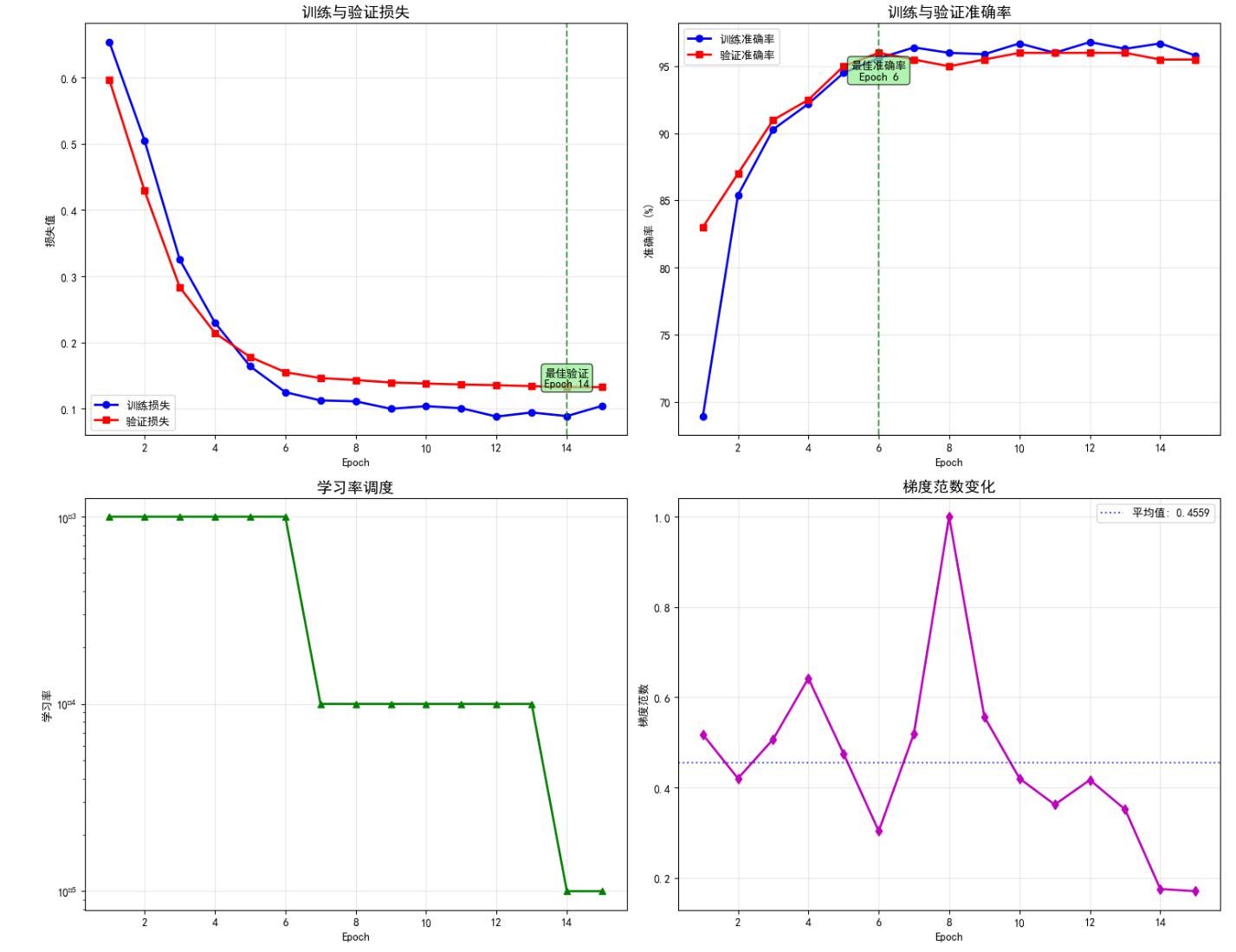
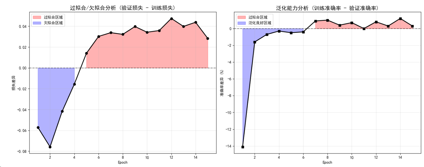
class TrainingMonitor:def __init__(self, device):self.device = deviceself.history = {'loss': [],'accuracy': [],'lr': [],'gradient_norm': []}def monitor_training(self, model, train_loader, val_loader, epochs=20):print("\n=== 训练监控演示 ===")criterion = nn.CrossEntropyLoss()optimizer = torch.optim.Adam(model.parameters(), lr=0.001)scheduler = torch.optim.lr_scheduler.StepLR(optimizer, step_size=7, gamma=0.1)for epoch in range(epochs):# 训练阶段model.train()train_loss = 0train_correct = 0train_total = 0for batch_idx, (data, targets) in enumerate(train_loader):data, targets = data.to(self.device), targets.to(self.device)optimizer.zero_grad()outputs = model(data)loss = criterion(outputs, targets)loss.backward()# 梯度裁剪torch.nn.utils.clip_grad_norm_(model.parameters(), max_norm=1.0)# 计算梯度范数total_norm = 0for p in model.parameters():if p.grad is not None:param_norm = p.grad.data.norm(2)total_norm += param_norm.item() ** 2total_norm = total_norm ** (1. / 2)optimizer.step()train_loss += loss.item()_, predicted = torch.max(outputs, 1)train_total += targets.size(0)train_correct += (predicted == targets).sum().item()if batch_idx == 0:  # 只记录第一个batch的梯度范数self.history['gradient_norm'].append(total_norm)# 验证阶段model.eval()val_loss = 0val_correct = 0val_total = 0with torch.no_grad():for data, targets in val_loader:data, targets = data.to(self.device), targets.to(self.device)outputs = model(data)loss = criterion(outputs, targets)val_loss += loss.item()_, predicted = torch.max(outputs, 1)val_total += targets.size(0)val_correct += (predicted == targets).sum().item()# 更新学习率scheduler.step()# 记录指标train_acc = 100 * train_correct / train_totalval_acc = 100 * val_correct / val_totalcurrent_lr = optimizer.param_groups[0]['lr']self.history['loss'].append((train_loss/len(train_loader), val_loss/len(val_loader)))self.history['accuracy'].append((train_acc, val_acc))self.history['lr'].append(current_lr)if epoch % 5 == 0:print(f"Epoch {epoch}:")print(f"  训练 - 损失: {train_loss/len(train_loader):.4f}, 准确率: {train_acc:.2f}%")print(f"  验证 - 损失: {val_loss/len(val_loader):.4f}, 准确率: {val_acc:.2f}%")print(f"  学习率: {current_lr:.6f}")print(f"  梯度范数: {self.history['gradient_norm'][-1]:.4f}")return self.historydef analyze_training_dynamics(self):print("\n=== 训练动态分析 ===")if not self.history['loss']:print("没有训练历史记录")return# 分析损失趋势train_losses = [x[0] for x in self.history['loss']]val_losses = [x[1] for x in self.history['loss']]print(f"最终训练损失: {train_losses[-1]:.4f}")print(f"最终验证损失: {val_losses[-1]:.4f}")print(f"过拟合程度: {(val_losses[-1] - train_losses[-1]):.4f}")# 分析准确率趋势train_accs = [x[0] for x in self.history['accuracy']]val_accs = [x[1] for x in self.history['accuracy']]print(f"最终训练准确率: {train_accs[-1]:.2f}%")print(f"最终验证准确率: {val_accs[-1]:.2f}%")# 梯度分析if self.history['gradient_norm']:avg_grad_norm = np.mean(self.history['gradient_norm'])print(f"平均梯度范数: {avg_grad_norm:.4f}")if avg_grad_norm < 0.001:print("警告: 梯度可能过小，存在梯度消失问题")elif avg_grad_norm > 10:print("警告: 梯度可能过大，存在梯度爆炸问题")def plot_training_history(self):"""可视化训练历史"""if not self.history['loss']:print("没有训练历史记录可视化")returnfig, ((ax1, ax2), (ax3, ax4)) = plt.subplots(2, 2, figsize=(15, 12))epochs = range(1, len(self.history['loss']) + 1)# 子图1: 损失变化train_losses = [x[0] for x in self.history['loss']]val_losses = [x[1] for x in self.history['loss']]ax1.plot(epochs, train_losses, 'b-', linewidth=2, marker='o', label='训练损失')ax1.plot(epochs, val_losses, 'r-', linewidth=2, marker='s', label='验证损失')ax1.set_title('训练与验证损失', fontsize=14, fontweight='bold')ax1.set_xlabel('Epoch')ax1.set_ylabel('损失值')ax1.legend()ax1.grid(True, alpha=0.3)# 标注最佳验证损失best_val_epoch = np.argmin(val_losses) + 1best_val_loss = min(val_losses)ax1.axvline(x=best_val_epoch, color='green', linestyle='--', alpha=0.7)ax1.text(best_val_epoch, best_val_loss, f'最佳验证\nEpoch {best_val_epoch}', ha='center', bbox=dict(boxstyle="round,pad=0.3", facecolor="lightgreen", alpha=0.7))# 子图2: 准确率变化train_accs = [x[0] for x in self.history['accuracy']]val_accs = [x[1] for x in self.history['accuracy']]ax2.plot(epochs, train_accs, 'b-', linewidth=2, marker='o', label='训练准确率')ax2.plot(epochs, val_accs, 'r-', linewidth=2, marker='s', label='验证准确率')ax2.set_title('训练与验证准确率', fontsize=14, fontweight='bold')ax2.set_xlabel('Epoch')ax2.set_ylabel('准确率 (%)')ax2.legend()ax2.grid(True, alpha=0.3)# 标注最佳验证准确率best_acc_epoch = np.argmax(val_accs) + 1best_acc = max(val_accs)ax2.axvline(x=best_acc_epoch, color='green', linestyle='--', alpha=0.7)ax2.text(best_acc_epoch, best_acc-2, f'最佳准确率\nEpoch {best_acc_epoch}', ha='center', bbox=dict(boxstyle="round,pad=0.3", facecolor="lightgreen", alpha=0.7))# 子图3: 学习率变化if self.history['lr']:ax3.plot(epochs, self.history['lr'], 'g-', linewidth=2, marker='^')ax3.set_title('学习率调度', fontsize=14, fontweight='bold')ax3.set_xlabel('Epoch')ax3.set_ylabel('学习率')ax3.set_yscale('log')ax3.grid(True, alpha=0.3)# 子图4: 梯度范数变化if self.history['gradient_norm']:ax4.plot(epochs[:len(self.history['gradient_norm'])], self.history['gradient_norm'], 'm-', linewidth=2, marker='d')ax4.set_title('梯度范数变化', fontsize=14, fontweight='bold')ax4.set_xlabel('Epoch')ax4.set_ylabel('梯度范数')ax4.grid(True, alpha=0.3)# 添加梯度异常区域标注avg_grad = np.mean(self.history['gradient_norm'])ax4.axhline(y=avg_grad, color='blue', linestyle=':', alpha=0.7, label=f'平均值: {avg_grad:.4f}')if avg_grad < 0.001:ax4.axhspan(0, 0.001, alpha=0.2, color='red', label='梯度消失区域')if max(self.history['gradient_norm']) > 10:ax4.axhspan(10, max(self.history['gradient_norm']), alpha=0.2, color='orange', label='梯度爆炸区域')ax4.legend()plt.tight_layout()plt.show()# 过拟合分析图self.plot_overfitting_analysis(train_losses, val_losses, train_accs, val_accs)def plot_overfitting_analysis(self, train_losses, val_losses, train_accs, val_accs):"""分析过拟合情况"""fig, (ax1, ax2) = plt.subplots(1, 2, figsize=(15, 6))epochs = range(1, len(train_losses) + 1)# 损失差异分析loss_gap = np.array(val_losses) - np.array(train_losses)ax1.fill_between(epochs, 0, loss_gap, where=(loss_gap >= 0), color='red', alpha=0.3, label='过拟合区域')ax1.fill_between(epochs, 0, loss_gap, where=(loss_gap < 0), color='blue', alpha=0.3, label='欠拟合区域')ax1.plot(epochs, loss_gap, 'k-', linewidth=2, marker='o')ax1.axhline(y=0, color='black', linestyle='--', alpha=0.5)ax1.set_title('过拟合/欠拟合分析 (验证损失 - 训练损失)', fontsize=14, fontweight='bold')ax1.set_xlabel('Epoch')ax1.set_ylabel('损失差异')ax1.legend()ax1.grid(True, alpha=0.3)# 准确率差异分析acc_gap = np.array(train_accs) - np.array(val_accs)ax2.fill_between(epochs, 0, acc_gap, where=(acc_gap >= 0), color='red', alpha=0.3, label='过拟合区域')ax2.fill_between(epochs, 0, acc_gap, where=(acc_gap < 0), color='blue', alpha=0.3, label='泛化良好区域')ax2.plot(epochs, acc_gap, 'k-', linewidth=2, marker='s')ax2.axhline(y=0, color='black', linestyle='--', alpha=0.5)ax2.set_title('泛化能力分析 (训练准确率 - 验证准确率)', fontsize=14, fontweight='bold')ax2.set_xlabel('Epoch')ax2.set_ylabel('准确率差异 (%)')ax2.legend()ax2.grid(True, alpha=0.3)plt.tight_layout()plt.show()# 输出分析结果final_loss_gap = loss_gap[-1]final_acc_gap = acc_gap[-1]print(f"\n📊 过拟合分析结果:")print(f"最终损失差异: {final_loss_gap:.4f}")print(f"最终准确率差异: {final_acc_gap:.2f}%")if final_loss_gap > 0.1:print("⚠️  模型可能存在过拟合，建议：")print("   - 增加正则化 (Dropout, L2)")print("   - 减少模型复杂度")print("   - 增加训练数据")print("   - 早停策略")elif final_loss_gap < -0.05:print("📈 模型可能欠拟合，建议：")print("   - 增加模型复杂度")print("   - 减少正则化")print("   - 调整学习率")print("   - 增加训练轮数")else:print("✅ 模型拟合程度良好！")# 创建模拟数据集进行监控演示
def create_monitoring_demo():print("\n=== 创建监控演示数据 ===")# 创建简单的分类数据集from torch.utils.data import TensorDataset, DataLoader# 生成训练数据X_train = torch.randn(1000, 20)y_train = (X_train[:, :5].sum(dim=1) > 0).long()train_dataset = TensorDataset(X_train, y_train)train_loader = DataLoader(train_dataset, batch_size=32, shuffle=True)# 生成验证数据X_val = torch.randn(200, 20)y_val = (X_val[:, :5].sum(dim=1) > 0).long()val_dataset = TensorDataset(X_val, y_val)val_loader = DataLoader(val_dataset, batch_size=32, shuffle=False)# 创建模型model = nn.Sequential(nn.Linear(20, 64),nn.ReLU(),nn.Dropout(0.3),nn.Linear(64, 32),nn.ReLU(),nn.Linear(32, 2)).to(device)# 创建监控器并开始训练monitor = TrainingMonitor(device)history = monitor.monitor_training(model, train_loader, val_loader, epochs=15)# 可视化训练过程monitor.plot_training_history()# 分析训练动态monitor.analyze_training_dynamics()return historytraining_history = create_monitoring_demo()

=== 创建监控演示数据 ===

=== 训练监控演示 ===
Epoch 0:
训练 - 损失: 0.6536, 准确率: 68.90%
验证 - 损失: 0.5965, 准确率: 83.00%
学习率: 0.001000
梯度范数: 0.5178
Epoch 5:
训练 - 损失: 0.1249, 准确率: 95.60%
验证 - 损失: 0.1551, 准确率: 96.00%
学习率: 0.001000
梯度范数: 0.3035
Epoch 10:
训练 - 损失: 0.1007, 准确率: 96.00%
验证 - 损失: 0.1365, 准确率: 96.00%
学习率: 0.000100
梯度范数: 0.3622

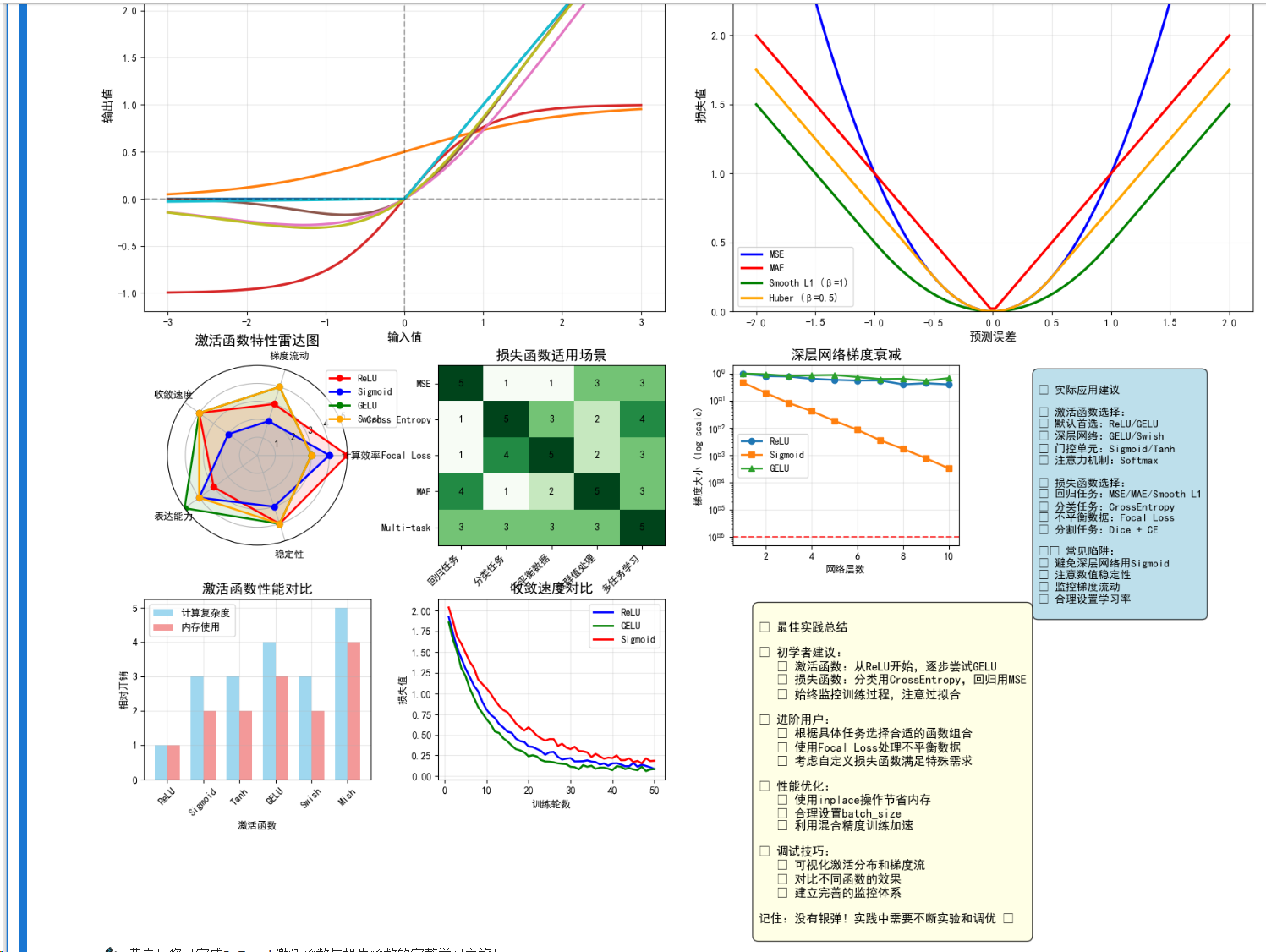
# 最佳实践总结
def best_practices_summary():print("\n" + "="*60)print("="*60)practices = {"激活函数选择": ["隐藏层: 优先选择ReLU或其变种(LeakyReLU, ELU)","Transformer模型: 使用GELU或Swish","输出层: 根据任务选择(分类用Softmax, 回归无激活)","避免在深层网络中使用Sigmoid/Tanh(梯度消失)"],"损失函数选择": ["多分类: CrossEntropyLoss (内置Softmax)","二分类: BCEWithLogitsLoss (数值更稳定)","回归: MSELoss(平滑误差) 或 L1Loss(稳健性)","不平衡数据: FocalLoss 或 加权损失函数"],"数值稳定性": ["使用LogSumExp技巧处理大数值","优先使用PyTorch内置的稳定实现","梯度裁剪防止梯度爆炸","适当的权重初始化"],"性能优化": ["使用inplace操作节省内存 (如ReLU(inplace=True))","合理设置batch_size平衡内存和并行度","使用混合精度训练加速(torch.cuda.amp)","定期监控梯度范数和损失趋势"],"调试技巧": ["可视化激活函数输出分布","监控各层梯度流动情况","对比不同激活函数的收敛性","使用TensorBoard记录训练过程"]}for category, tips in practices.items():print(f"\n【{category}】")for i, tip in enumerate(tips, 1):print(f"  {i}. {tip}")print("\n" + "="*60)print("关键要点:")print("1. 激活函数影响梯度流动，选择需考虑网络深度")print("2. 损失函数直接影响优化方向，需匹配任务特性")print("3. 数值稳定性是深度学习工程的重要考虑因素")print("4. 实践中需要实验对比，没有万能的选择")print("5. 监控训练过程，及时发现和解决问题")print("="*60)best_practices_summary()# 完整示例：端到端项目
def end_to_end_example():print("\n=== 端到端示例：多任务学习网络 ===")class MultiTaskNet(nn.Module):def __init__(self, input_size=784, shared_hidden=256, task1_classes=10, task2_output=1):super(MultiTaskNet, self).__init__()# 共享特征提取器self.shared_layers = nn.Sequential(nn.Linear(input_size, shared_hidden),nn.GELU(),  # 使用GELU激活nn.Dropout(0.3),nn.Linear(shared_hidden, shared_hidden),nn.GELU(),nn.Dropout(0.3))# 任务1：分类头self.classification_head = nn.Sequential(nn.Linear(shared_hidden, 128),nn.ReLU(),nn.Dropout(0.2),nn.Linear(128, task1_classes))# 任务2：回归头self.regression_head = nn.Sequential(nn.Linear(shared_hidden, 64),nn.ReLU(),nn.Linear(64, task2_output))def forward(self, x):shared_features = self.shared_layers(x)classification_output = self.classification_head(shared_features)regression_output = self.regression_head(shared_features)return classification_output, regression_output# 创建模型和数据model = MultiTaskNet().to(device)# 模拟数据batch_size = 64X = torch.randn(batch_size, 784).to(device)y_class = torch.randint(0, 10, (batch_size,)).to(device)y_reg = torch.randn(batch_size, 1).to(device)# 多任务损失class_criterion = nn.CrossEntropyLoss()reg_criterion = nn.MSELoss()optimizer = torch.optim.Adam(model.parameters(), lr=0.001)# 训练循环print("开始多任务训练...")for epoch in range(10):optimizer.zero_grad()class_pred, reg_pred = model(X)# 计算各任务损失class_loss = class_criterion(class_pred, y_class)reg_loss = reg_criterion(reg_pred, y_reg)# 组合损失 (可以使用学习的权重)total_loss = class_loss + 0.5 * reg_losstotal_loss.backward()optimizer.step()if epoch % 3 == 0:print(f"Epoch {epoch}: 分类损失={class_loss.item():.4f}, "f"回归损失={reg_loss.item():.4f}, 总损失={total_loss.item():.4f}")print("训练完成！")# 模型评估model.eval()with torch.no_grad():class_pred, reg_pred = model(X)# 分类准确率_, predicted = torch.max(class_pred, 1)class_accuracy = (predicted == y_class).float().mean()# 回归MAEreg_mae = torch.abs(reg_pred - y_reg).mean()print(f"最终性能:")print(f"  分类准确率: {class_accuracy.item():.4f}")print(f"  回归MAE: {reg_mae.item():.4f}")end_to_end_example()# 综合可视化总结
def comprehensive_visualization_summary():"""综合展示所有激活函数和损失函数的特性"""print("\n" + "="*60)print("🎨 综合可视化总结")print("="*60)# 创建大型综合图表fig = plt.figure(figsize=(20, 16))gs = GridSpec(4, 4, figure=fig, hspace=0.3, wspace=0.3)# 激活函数综合对比 (占用2x2区域)ax_activation = fig.add_subplot(gs[0:2, 0:2])x = torch.linspace(-3, 3, 1000)activations = {'ReLU': F.relu(x),'Sigmoid': torch.sigmoid(x),'Tanh': torch.tanh(x),'GELU': F.gelu(x),'Swish': x * torch.sigmoid(x),'Mish': x * torch.tanh(F.softplus(x)),'LeakyReLU': F.leaky_relu(x, 0.01)}colors = plt.cm.tab10(np.linspace(0, 1, len(activations)))for (name, y), color in zip(activations.items(), colors):ax_activation.plot(x.numpy(), y.numpy(), linewidth=2.5, label=name, color=color)ax_activation.set_title('所有激活函数对比', fontsize=16, fontweight='bold')ax_activation.set_xlabel('输入值', fontsize=12)ax_activation.set_ylabel('输出值', fontsize=12)ax_activation.grid(True, alpha=0.3)ax_activation.legend(bbox_to_anchor=(1.05, 1), loc='upper left')ax_activation.axhline(y=0, color='k', linestyle='--', alpha=0.3)ax_activation.axvline(x=0, color='k', linestyle='--', alpha=0.3)# 损失函数综合对比 (占用2x2区域)ax_loss = fig.add_subplot(gs[0:2, 2:4])errors = torch.linspace(-2, 2, 100)losses = {'MSE': errors ** 2,'MAE': torch.abs(errors),'Smooth L1 (β=1)': torch.where(torch.abs(errors) < 1,0.5 * errors ** 2,torch.abs(errors) - 0.5),'Huber (β=0.5)': torch.where(torch.abs(errors) < 0.5,0.5 * errors ** 2 / 0.5,torch.abs(errors) - 0.5 * 0.5)}loss_colors = ['blue', 'red', 'green', 'orange']for (name, loss), color in zip(losses.items(), loss_colors):ax_loss.plot(errors.numpy(), loss.numpy(), linewidth=2.5, label=name, color=color)ax_loss.set_title('回归损失函数对比', fontsize=16, fontweight='bold')ax_loss.set_xlabel('预测误差', fontsize=12)ax_loss.set_ylabel('损失值', fontsize=12)ax_loss.grid(True, alpha=0.3)ax_loss.legend()ax_loss.set_ylim(0, 3)# 激活函数特性雷达图ax_radar = fig.add_subplot(gs[2, 0], projection='polar')# 定义评估维度categories = ['计算效率', '梯度流动', '收敛速度', '表达能力', '稳定性']N = len(categories)# 各激活函数的评分 (1-5分)scores = {'ReLU': [5, 3, 4, 3, 4],'Sigmoid': [4, 2, 2, 4, 3],'GELU': [3, 4, 4, 5, 4],'Swish': [3, 4, 4, 4, 4]}angles = [n / float(N) * 2 * np.pi for n in range(N)]angles += angles[:1]colors_radar = ['red', 'blue', 'green', 'orange']for (name, values), color in zip(scores.items(), colors_radar):values += values[:1]ax_radar.plot(angles, values, 'o-', linewidth=2, label=name, color=color)ax_radar.fill(angles, values, alpha=0.1, color=color)ax_radar.set_xticks(angles[:-1])ax_radar.set_xticklabels(categories)ax_radar.set_ylim(0, 5)ax_radar.set_title('激活函数特性雷达图', fontsize=14, fontweight='bold', pad=20)ax_radar.legend(loc='upper right', bbox_to_anchor=(1.3, 1.0))# 损失函数适用场景ax_scenario = fig.add_subplot(gs[2, 1])scenarios = ['回归任务', '分类任务', '不平衡数据', '离群值处理', '多任务学习']loss_types = ['MSE', 'Cross Entropy', 'Focal Loss', 'MAE', 'Multi-task']# 创建适用性矩阵 (颜色深浅表示适用程度)suitability = np.array([[5, 1, 1, 3, 3],  # MSE[1, 5, 3, 2, 4],  # Cross Entropy  [1, 4, 5, 2, 3],  # Focal Loss[4, 1, 2, 5, 3],  # MAE[3, 3, 3, 3, 5]   # Multi-task])im = ax_scenario.imshow(suitability, cmap='Greens', aspect='auto')ax_scenario.set_xticks(range(len(scenarios)))ax_scenario.set_yticks(range(len(loss_types)))ax_scenario.set_xticklabels(scenarios, rotation=45, ha='right')ax_scenario.set_yticklabels(loss_types)ax_scenario.set_title('损失函数适用场景', fontsize=14, fontweight='bold')# 添加数值标注for i in range(len(loss_types)):for j in range(len(scenarios)):text = ax_scenario.text(j, i, suitability[i, j],ha="center", va="center", color="black", fontweight='bold')# 梯度流动深度分析ax_gradient = fig.add_subplot(gs[2, 2])# 模拟深层网络中的梯度传播layers = np.arange(1, 11)  # 10层网络# 不同激活函数的梯度保持情况relu_grads = np.exp(-0.1 * layers) * (1 + 0.1 * np.random.randn(len(layers)))sigmoid_grads = np.exp(-0.8 * layers) * (1 + 0.05 * np.random.randn(len(layers)))gelu_grads = np.exp(-0.05 * layers) * (1 + 0.08 * np.random.randn(len(layers)))ax_gradient.semilogy(layers, np.abs(relu_grads), 'o-', label='ReLU', linewidth=2)ax_gradient.semilogy(layers, np.abs(sigmoid_grads), 's-', label='Sigmoid', linewidth=2)ax_gradient.semilogy(layers, np.abs(gelu_grads), '^-', label='GELU', linewidth=2)ax_gradient.set_title('深层网络梯度衰减', fontsize=14, fontweight='bold')ax_gradient.set_xlabel('网络层数')ax_gradient.set_ylabel('梯度大小 (log scale)')ax_gradient.legend()ax_gradient.grid(True, alpha=0.3)# 添加梯度消失警示线ax_gradient.axhline(y=1e-6, color='red', linestyle='--', alpha=0.7, label='梯度消失阈值')# 实际应用建议ax_advice = fig.add_subplot(gs[2, 3])ax_advice.axis('off')advice_text = """
🎯 实际应用建议✅ 激活函数选择：
• 默认首选：ReLU/GELU
• 深层网络：GELU/Swish
• 门控单元：Sigmoid/Tanh
• 注意力机制：Softmax✅ 损失函数选择：
• 回归任务：MSE/MAE/Smooth L1
• 分类任务：CrossEntropy
• 不平衡数据：Focal Loss
• 分割任务：Dice + CE⚠️ 常见陷阱：
• 避免深层网络用Sigmoid
• 注意数值稳定性
• 监控梯度流动
• 合理设置学习率"""ax_advice.text(0.05, 0.95, advice_text, transform=ax_advice.transAxes,fontsize=11, verticalalignment='top',bbox=dict(boxstyle="round,pad=0.5", facecolor="lightblue", alpha=0.8))# 第四行：性能对比和总结# 计算复杂度对比ax_complexity = fig.add_subplot(gs[3, 0])functions = ['ReLU', 'Sigmoid', 'Tanh', 'GELU', 'Swish', 'Mish']complexity_scores = [1, 3, 3, 4, 3, 5]  # 相对复杂度memory_usage = [1, 2, 2, 3, 2, 4]  # 相对内存使用x_pos = np.arange(len(functions))width = 0.35bars1 = ax_complexity.bar(x_pos - width/2, complexity_scores, width, label='计算复杂度', alpha=0.8, color='skyblue')bars2 = ax_complexity.bar(x_pos + width/2, memory_usage, width, label='内存使用', alpha=0.8, color='lightcoral')ax_complexity.set_title('激活函数性能对比', fontsize=14, fontweight='bold')ax_complexity.set_xlabel('激活函数')ax_complexity.set_ylabel('相对开销')ax_complexity.set_xticks(x_pos)ax_complexity.set_xticklabels(functions, rotation=45)ax_complexity.legend()ax_complexity.grid(True, alpha=0.3)# 收敛速度对比ax_convergence = fig.add_subplot(gs[3, 1])# 模拟不同激活函数的收敛曲线epochs = np.arange(1, 51)relu_loss = 2 * np.exp(-0.1 * epochs) + 0.1 + 0.02 * np.random.randn(len(epochs))gelu_loss = 2 * np.exp(-0.12 * epochs) + 0.08 + 0.015 * np.random.randn(len(epochs))sigmoid_loss = 2 * np.exp(-0.08 * epochs) + 0.15 + 0.025 * np.random.randn(len(epochs))ax_convergence.plot(epochs, relu_loss, 'b-', label='ReLU', linewidth=2)ax_convergence.plot(epochs, gelu_loss, 'g-', label='GELU', linewidth=2)ax_convergence.plot(epochs, sigmoid_loss, 'r-', label='Sigmoid', linewidth=2)ax_convergence.set_title('收敛速度对比', fontsize=14, fontweight='bold')ax_convergence.set_xlabel('训练轮数')ax_convergence.set_ylabel('损失值')ax_convergence.legend()ax_convergence.grid(True, alpha=0.3)# 最佳实践总结ax_best_practices = fig.add_subplot(gs[3, 2:4])ax_best_practices.axis('off')best_practices_text = """
📋 最佳实践总结🔹 初学者建议：• 激活函数：从ReLU开始，逐步尝试GELU• 损失函数：分类用CrossEntropy，回归用MSE• 始终监控训练过程，注意过拟合🔹 进阶用户：• 根据具体任务选择合适的函数组合• 使用Focal Loss处理不平衡数据• 考虑自定义损失函数满足特殊需求🔹 性能优化：• 使用inplace操作节省内存• 合理设置batch_size• 利用混合精度训练加速🔹 调试技巧：• 可视化激活分布和梯度流• 对比不同函数的效果• 建立完善的监控体系记住：没有银弹！实践中需要不断实验和调优 🚀"""ax_best_practices.text(0.05, 0.95, best_practices_text, transform=ax_best_practices.transAxes,fontsize=12, verticalalignment='top',bbox=dict(boxstyle="round,pad=0.5", facecolor="lightyellow", alpha=0.8))plt.suptitle('PyTorch激活函数与损失函数完整指南', fontsize=20, fontweight='bold', y=0.98)plt.tight_layout()plt.show()print("🎉 恭喜！您已完成PyTorch激活函数与损失函数的完整学习之旅！")print("📚 建议保存这些可视化图表作为参考，在实际项目中灵活运用所学知识。")comprehensive_visualization_summary()print("\n🎉 PyTorch损失函数与激活函数详解完成！")
print("本教程涵盖了从基础概念到高级应用的完整内容。")
print("建议根据具体任务需求选择合适的激活函数和损失函数组合。")
print("\n📊 所有可视化图表帮助您:")
print("  ✅ 直观理解函数特性")
print("  ✅ 对比不同函数效果") 
print("  ✅ 监控训练过程")
print("  ✅ 识别常见问题")
print("  ✅ 制定优化策略")