当前位置：首页 > web >正文

SOC估算方法-蜣螂优化算法结合极限学习

web 2025/8/24 7:20:17

原始论文名称叫A combined improved dung beetle optimization and extreme learning machine framework for precise SOC estimation

关键创新

改进的粪金龟优化算法（IDBO）：
- 通过三种策略增强了传统的粪金龟优化算法（DBO），使其能有效避免局部最优并提升全局搜索能力：
  - 圆形混沌映射（Circle Chaotic Mapping）：改进了种群初始化，确保了初始化种群的分布均匀，进而增加了解的多样性，避免了标准DBO算法中可能出现的不均匀初始种群问题。
  - 黄金正弦策略（Golden Sine Strategy）：在“滚动球”粪金龟的移动更新中采用正弦函数替代常数系数，增强了全局搜索能力，帮助算法更好地探索解空间。
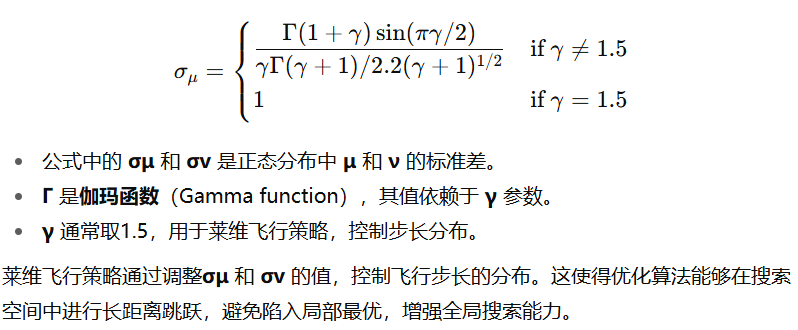
  - 莱维飞行策略（Levy Flight Strategy）：通过莱维分布实现随机的远距离搜索，帮助算法避免过早收敛到局部最优，提升了全局搜索能力。
极限学习机（ELM）：
- 极限学习机（ELM）是一种具有单隐层的前馈神经网络，具备快速学习的特性。与传统的神经网络相比，ELM的训练过程不依赖于反向传播算法，而是通过解析解来直接计算输出层的权重。
- 该模型通过使用IDBO算法优化ELM网络的输入权重和隐藏层偏置，提升了SOC预测的精度。

IDBO-ELM 算法流程

数据预处理：首先对锂电池的SOC数据进行归一化处理，并将数据分为训练集和测试集。
种群初始化：使用圆形混沌映射初始化粪金龟种群，确保种群的初始分布均匀，提高算法的多样性。
优化过程：利用IDBO算法的三个策略（圆形混沌映射、黄金正弦策略、莱维飞行策略）迭代优化ELM的超参数，特别是输入层的权重和偏置。
模型构建：通过优化得到的最优超参数构建ELM模型，进而进行SOC预测。

公式解析

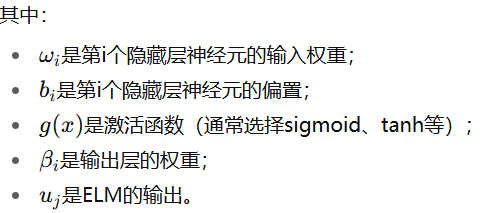
ELM模型公式：

对于ELM模型，假设输入层有n个神经元，隐藏层有L个神经元，输出层有m个神经元。给定Q个训练样本(xi,yi)，其中xi表示输入数据，yi表示输出数据。ELM的数学模型如下：

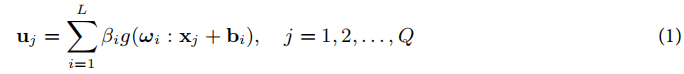
通过最小化训练误差，ELM的目标是通过解最小二乘法来求解输出层的权重β。

训练目标函数为：

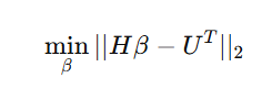
其中，H是隐藏层输出矩阵，U是训练样本的目标输出。

最终，通过最小二乘解计算输出层权重β：

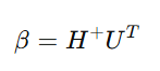
其中，H+是H的摩尔－彭若斯广义逆。

"""
Extreme Learning Machine (ELM) implementation for SOC estimation
"""import numpy as np
from sklearn.preprocessing import StandardScaler
from typing import Tuple, Optionalclass ExtremeLearningMachine:def __init__(self,input_size: int,hidden_size: int,output_size: int,activation: str = 'sigmoid',random_state: Optional[int] = None):"""Initialize Extreme Learning MachineArgs:input_size: Number of input featureshidden_size: Number of hidden neuronsoutput_size: Number of output neuronsactivation: Activation function ('sigmoid', 'tanh', 'relu')random_state: Random seed for reproducibility"""self.input_size = input_sizeself.hidden_size = hidden_sizeself.output_size = output_sizeself.activation = activation# Set random seed if providedif random_state is not None:np.random.seed(random_state)# Initialize input weights and biases randomly# These are the parameters that will be optimized by IDBOself.input_weights = np.random.uniform(-1, 1, (self.input_size, self.hidden_size))self.biases = np.random.uniform(-1, 1, self.hidden_size)# Output weights will be calculated analyticallyself.output_weights = None# Scaling for input normalizationself.scaler = StandardScaler()def _activate(self, x: np.ndarray) -> np.ndarray:"""Apply activation functionArgs:x: Input arrayReturns:Activated output"""if self.activation == 'sigmoid':return 1.0 / (1.0 + np.exp(-x))elif self.activation == 'tanh':return np.tanh(x)elif self.activation == 'relu':return np.maximum(0, x)else:raise ValueError(f"Unsupported activation function: {self.activation}")def _calculate_hidden_layer_output(self, X: np.ndarray) -> np.ndarray:"""Calculate the output of the hidden layerArgs:X: Input data of shape (n_samples, input_size)Returns:Hidden layer output of shape (n_samples, hidden_size)"""# Calculate the weighted sumweighted_sum = np.dot(X, self.input_weights) + self.biases# Apply activation functionH = self._activate(weighted_sum)return Hdef fit(self, X: np.ndarray, y: np.ndarray) -> None:"""Train the ELM modelArgs:X: Training data of shape (n_samples, input_size)y: Target values of shape (n_samples, output_size)"""# Scale input dataX_scaled = self.scaler.fit_transform(X)# Calculate hidden layer outputH = self._calculate_hidden_layer_output(X_scaled)# Calculate output weights using Moore-Penrose pseudoinverse# This is the analytical solution that makes ELM fastH_pinv = np.linalg.pinv(H)self.output_weights = np.dot(H_pinv, y)def predict(self, X: np.ndarray) -> np.ndarray:"""Make predictions using the trained ELM modelArgs:X: Input data of shape (n_samples, input_size)Returns:Predictions of shape (n_samples, output_size)"""# Scale input dataX_scaled = self.scaler.transform(X)# Calculate hidden layer outputH = self._calculate_hidden_layer_output(X_scaled)# Calculate predictionspredictions = np.dot(H, self.output_weights)return predictionsdef evaluate(self, X: np.ndarray, y: np.ndarray) -> Tuple[float, float, float]:"""Evaluate the model performanceArgs:X: Test datay: True valuesReturns:Tuple of (RMSE, MAE, R²)"""y_pred = self.predict(X)# Calculate Root Mean Squared Error (RMSE)rmse = np.sqrt(np.mean((y_pred - y) ** 2))# Calculate Mean Absolute Error (MAE)mae = np.mean(np.abs(y_pred - y))# Calculate R² (coefficient of determination)ss_total = np.sum((y - np.mean(y)) ** 2)ss_residual = np.sum((y - y_pred) ** 2)r2 = 1 - (ss_residual / ss_total)return rmse, mae, r2def get_params(self) -> np.ndarray:"""Get the model parameters (input weights and biases) as a flat arrayReturns:Flattened array of parameters"""return np.concatenate([self.input_weights.flatten(), self.biases])def set_params(self, params: np.ndarray) -> None:"""Set the model parameters from a flat arrayArgs:params: Flattened array of parameters"""# Split the parameters back into weights and biasesinput_weights_size = self.input_size * self.hidden_sizeself.input_weights = params[:input_weights_size].reshape(self.input_size, self.hidden_size)self.biases = params[input_weights_size:]

改进的DBO算法：

圆形混沌映射：这一步用于优化DBO种群的初始化，使其分布更加均匀。其更新公式为：

其中，a1,a2,a3是常数，控制混沌映射的行为，xn是当前的位置。

def _circle_chaotic_initialization(self) -> np.ndarray:"""Initialize population using circle chaotic mapping for better diversityas described in the paper (equation 5)Returns:Initialized population"""population = np.zeros((self.population_size, self.dimensions))# Initialize chaotic variablesz = np.random.random(self.population_size)for i in range(self.population_size):# Generate chaotic sequence using circle mapx = np.zeros(self.dimensions)z_i = z[i]for j in range(self.dimensions):# Circle chaotic map equation: z_{n+1} = (z_n + Ω - K/(2π) * sin(2πz_n)) mod 1# Using simplified parameters: Ω = 0.5, K = 1z_i = (z_i + 0.5 - (1/(2*np.pi)) * np.sin(2*np.pi*z_i)) % 1x[j] = z_i# Map to search spacepopulation[i] = self.lower_bound + (self.upper_bound - self.lower_bound) * xreturn population

黄金正弦策略：更新“滚动球”粪金龟的位置时，采用正弦函数代替常数系数，以增加解空间的探索。位置更新公式为：

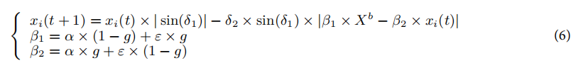
其中，δ1和δ2是随机数，β1和β2是黄金比例系数，Xb是当前最佳个体的位置。

def _update_rolling_factor(self, iteration: int) -> None:"""Update rolling factor adaptively based on iteration progressArgs:iteration: Current iteration number"""# Linear decrease from 0.9 to 0.1self.rolling_factor = 0.9 - 0.8 * (iteration / self.max_iterations)

莱维飞行策略：用于避免粪金龟“偷窃”个体位置过早收敛到局部最优。其更新公式为：

其中，Levy(λ)表示遵循莱维分布的随机搜索路径，⊕是点积运算，ω是步长。

    def _levy_flight(self) -> np.ndarray:"""Generate step using Lévy flight distributionas described in the paper (equations 7-9)Returns:Step vector following Lévy distribution"""# Implementation of Lévy flightsigma = (scipy.special.gamma(1 + self.levy_alpha) * np.sin(np.pi * self.levy_alpha / 2) / (scipy.special.gamma((1 + self.levy_alpha) / 2) * self.levy_alpha * 2**((self.levy_alpha - 1) / 2)))**(1 / self.levy_alpha)# Generate step from Lévy distributionu = np.random.normal(0, sigma, self.dimensions)v = np.random.normal(0, 1, self.dimensions)step = u / (np.abs(v)**(1 / self.levy_alpha))return step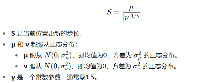

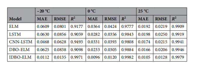
评价标准

MAE RMSE R2

完整的代码在下面

elm.py

"""
Extreme Learning Machine (ELM) implementation for SOC estimation
"""import numpy as np
from sklearn.preprocessing import StandardScaler
from typing import Tuple, Optionalclass ExtremeLearningMachine:def __init__(self,input_size: int,hidden_size: int,output_size: int,activation: str = 'sigmoid',random_state: Optional[int] = None):"""Initialize Extreme Learning MachineArgs:input_size: Number of input featureshidden_size: Number of hidden neuronsoutput_size: Number of output neuronsactivation: Activation function ('sigmoid', 'tanh', 'relu')random_state: Random seed for reproducibility"""self.input_size = input_sizeself.hidden_size = hidden_sizeself.output_size = output_sizeself.activation = activation# Set random seed if providedif random_state is not None:np.random.seed(random_state)# Initialize input weights and biases randomly# These are the parameters that will be optimized by IDBOself.input_weights = np.random.uniform(-1, 1, (self.input_size, self.hidden_size))self.biases = np.random.uniform(-1, 1, self.hidden_size)# Output weights will be calculated analyticallyself.output_weights = None# Scaling for input normalizationself.scaler = StandardScaler()def _activate(self, x: np.ndarray) -> np.ndarray:"""Apply activation functionArgs:x: Input arrayReturns:Activated output"""if self.activation == 'sigmoid':return 1.0 / (1.0 + np.exp(-x))elif self.activation == 'tanh':return np.tanh(x)elif self.activation == 'relu':return np.maximum(0, x)else:raise ValueError(f"Unsupported activation function: {self.activation}")def _calculate_hidden_layer_output(self, X: np.ndarray) -> np.ndarray:"""Calculate the output of the hidden layerArgs:X: Input data of shape (n_samples, input_size)Returns:Hidden layer output of shape (n_samples, hidden_size)"""# Calculate the weighted sumweighted_sum = np.dot(X, self.input_weights) + self.biases# Apply activation functionH = self._activate(weighted_sum)return Hdef fit(self, X: np.ndarray, y: np.ndarray) -> None:"""Train the ELM modelArgs:X: Training data of shape (n_samples, input_size)y: Target values of shape (n_samples, output_size)"""# Scale input dataX_scaled = self.scaler.fit_transform(X)# Calculate hidden layer outputH = self._calculate_hidden_layer_output(X_scaled)# Calculate output weights using Moore-Penrose pseudoinverse# This is the analytical solution that makes ELM fastH_pinv = np.linalg.pinv(H)self.output_weights = np.dot(H_pinv, y)def predict(self, X: np.ndarray) -> np.ndarray:"""Make predictions using the trained ELM modelArgs:X: Input data of shape (n_samples, input_size)Returns:Predictions of shape (n_samples, output_size)"""# Scale input dataX_scaled = self.scaler.transform(X)# Calculate hidden layer outputH = self._calculate_hidden_layer_output(X_scaled)# Calculate predictionspredictions = np.dot(H, self.output_weights)return predictionsdef evaluate(self, X: np.ndarray, y: np.ndarray) -> Tuple[float, float, float]:"""Evaluate the model performanceArgs:X: Test datay: True valuesReturns:Tuple of (RMSE, MAE, R²)"""y_pred = self.predict(X)# Calculate Root Mean Squared Error (RMSE)rmse = np.sqrt(np.mean((y_pred - y) ** 2))# Calculate Mean Absolute Error (MAE)mae = np.mean(np.abs(y_pred - y))# Calculate R² (coefficient of determination)ss_total = np.sum((y - np.mean(y)) ** 2)ss_residual = np.sum((y - y_pred) ** 2)r2 = 1 - (ss_residual / ss_total)return rmse, mae, r2def get_params(self) -> np.ndarray:"""Get the model parameters (input weights and biases) as a flat arrayReturns:Flattened array of parameters"""return np.concatenate([self.input_weights.flatten(), self.biases])def set_params(self, params: np.ndarray) -> None:"""Set the model parameters from a flat arrayArgs:params: Flattened array of parameters"""# Split the parameters back into weights and biasesinput_weights_size = self.input_size * self.hidden_sizeself.input_weights = params[:input_weights_size].reshape(self.input_size, self.hidden_size)self.biases = params[input_weights_size:]

idbo_elm_soc.py

"""
Combined Improved Dung Beetle Optimization (IDBO) and Extreme Learning Machine (ELM) framework
for precise SOC estimation of batteriesImplementation based on the paper:
"A combined improved dung beetle optimization and extreme learning machine framework for precise SOC estimation"
"""import numpy as np
import matplotlib.pyplot as plt
from sklearn.model_selection import train_test_split
from sklearn.preprocessing import MinMaxScaler
import pandas as pd
from typing import Tuple, List, Dict, Any, Optionalfrom improved_dbo import ImprovedDungBeetleOptimizer
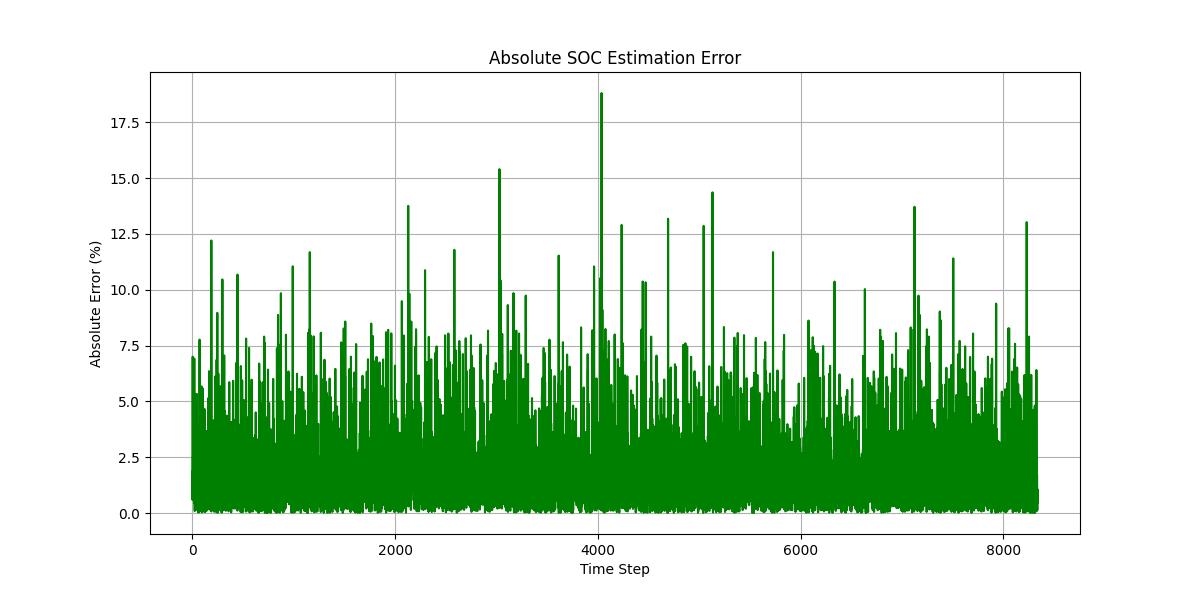
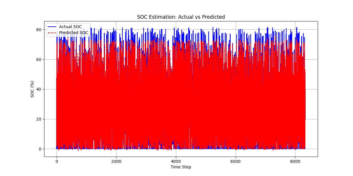
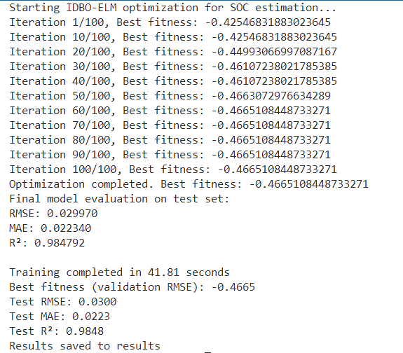
from elm import ExtremeLearningMachineclass IDBO_ELM_SOC:def __init__(self,hidden_neurons: int = 20,activation: str = 'sigmoid',population_size: int = 30,max_iterations: int = 100,initial_rolling_factor: float = 0.5,communication_probability: float = 0.3,elite_group_size: int = 5,opposition_probability: float = 0.1,levy_alpha: float = 1.5,golden_ratio: float = 1.618,random_state: Optional[int] = None):"""Initialize the IDBO-ELM framework for SOC estimationArgs:hidden_neurons: Number of hidden neurons in ELMactivation: Activation function for ELMpopulation_size: Population size for IDBOmax_iterations: Maximum iterations for IDBOinitial_rolling_factor: Initial factor for rolling behaviorcommunication_probability: Probability of communicationelite_group_size: Size of elite group in IDBOopposition_probability: Probability of opposition-based learninglevy_alpha: Parameter for Lévy flightgolden_ratio: Golden ratio for sine strategyrandom_state: Random seed for reproducibility"""self.hidden_neurons = hidden_neuronsself.activation = activationself.population_size = population_sizeself.max_iterations = max_iterationsself.initial_rolling_factor = initial_rolling_factorself.communication_probability = communication_probabilityself.elite_group_size = elite_group_sizeself.opposition_probability = opposition_probabilityself.levy_alpha = levy_alphaself.golden_ratio = golden_ratioself.random_state = random_state# These will be initialized later when data dimensions are knownself.elm = Noneself.optimizer = Noneself.input_size = Noneself.output_size = None# For storing resultsself.best_params = Noneself.best_fitness = Noneself.convergence_curve = None# Scalers for data normalization (0-1 range as mentioned in the paper)self.X_scaler = MinMaxScaler(feature_range=(0, 1))self.y_scaler = MinMaxScaler(feature_range=(0, 1))def _objective_function(self, params: np.ndarray) -> float:"""Objective function for IDBO optimizationEvaluates ELM performance with given parameters (input weights and biases)Args:params: Flattened array of ELM parameters (input weights and biases)Returns:Error metric (combined RMSE, MAE, R²) to be minimized"""# Set ELM parameters (input weights and biases)self.elm.set_params(params)# Train ELM with current parameters (this calculates output weights β analytically)self.elm.fit(self.X_train_scaled, self.y_train_scaled)# Predict on validation sety_pred = self.elm.predict(self.X_val_scaled)# Calculate error metricsrmse, mae, r2 = self._calculate_metrics(y_pred, self.y_val_scaled)# Combined fitness function (optimized weights)# Lower RMSE and MAE are better, higher R² is betterfitness = 0.6 * rmse + 0.3 * mae - 0.5 * r2return fitnessdef _calculate_metrics(self, y_pred: np.ndarray, y_true: np.ndarray) -> Tuple[float, float, float]:"""Calculate evaluation metricsArgs:y_pred: Predicted valuesy_true: True valuesReturns:Tuple of (RMSE, MAE, R²)"""# Root Mean Squared Errorrmse = np.sqrt(np.mean((y_pred - y_true) ** 2))# Mean Absolute Errormae = np.mean(np.abs(y_pred - y_true))# R² score with protection against division by zeross_total = np.sum((y_true - np.mean(y_true)) ** 2)ss_residual = np.sum((y_true - y_pred) ** 2)# Check if ss_total is close to zero (constant target values)if ss_total < 1e-10:# If target values are constant, R² is undefined# Return 0 or 1 based on prediction accuracyif ss_residual < 1e-10:r2 = 1.0  # Perfect predictionelse:r2 = 0.0  # Imperfect predictionelse:r2 = 1 - (ss_residual / ss_total)# Clip R² to valid range [-1, 1]r2 = np.clip(r2, -1.0, 1.0)return rmse, mae, r2def preprocess_data(self, X: np.ndarray, y: np.ndarray) -> Tuple[np.ndarray, np.ndarray, np.ndarray, np.ndarray, np.ndarray, np.ndarray]:"""Preprocess the data for training and testingNormalizes data to [0,1] range as mentioned in the paperArgs:X: Input featuresy: Target values (SOC)Returns:Tuple of (X_train, X_val, X_test, y_train, y_val, y_test)"""# Check for NaN values and replace themif np.isnan(X).any():print(f"Warning: Found {np.isnan(X).sum()} NaN values in features. Replacing with zeros.")X = np.nan_to_num(X, nan=0.0)if np.isnan(y).any():print(f"Warning: Found {np.isnan(y).sum()} NaN values in target. Replacing with zeros.")y = np.nan_to_num(y, nan=0.0)# Check for infinite values and replace themif np.isinf(X).any():print(f"Warning: Found {np.isinf(X).sum()} infinite values in features. Replacing with large values.")X = np.nan_to_num(X, posinf=1e10, neginf=-1e10)if np.isinf(y).any():print(f"Warning: Found {np.isinf(y).sum()} infinite values in target. Replacing with boundary values.")y = np.nan_to_num(y, posinf=100.0, neginf=0.0)# Scale input features and target values to [0,1] rangeX_scaled = self.X_scaler.fit_transform(X)y_scaled = self.y_scaler.fit_transform(y.reshape(-1, 1))# Split data into training and testing sets (80% train, 20% test)X_train, X_test, y_train, y_test = train_test_split(X_scaled, y_scaled, test_size=0.2, random_state=self.random_state)# Further split training data into training and validation sets (80% train, 20% validation)X_train, X_val, y_train, y_val = train_test_split(X_train, y_train, test_size=0.2, random_state=self.random_state)return X_train, X_val, X_test, y_train, y_val, y_testdef fit(self, X: np.ndarray, y: np.ndarray) -> Dict[str, Any]:"""Train the IDBO-ELM framework following the paper's algorithmArgs:X: Input featuresy: Target values (SOC)Returns:Dictionary with training results"""# Step 1: Get data dimensionsself.input_size = X.shape[1]self.output_size = 1  # SOC is a single value# Step 2: Preprocess data (normalize to [0,1] range)self.X_train_scaled, self.X_val_scaled, self.X_test_scaled, \self.y_train_scaled, self.y_val_scaled, self.y_test_scaled = self.preprocess_data(X, y)print(f"Data preprocessed. Training samples: {self.X_train_scaled.shape[0]}, "f"Validation samples: {self.X_val_scaled.shape[0]}, "f"Test samples: {self.X_test_scaled.shape[0]}")# Step 3: Initialize ELM with random input weights and biasesself.elm = ExtremeLearningMachine(input_size=self.input_size,hidden_size=self.hidden_neurons,output_size=self.output_size,activation=self.activation,random_state=self.random_state)# Calculate parameter dimensions for IDBO# Parameters to optimize: input weights (input_size * hidden_neurons) and biases (hidden_neurons)param_size = self.input_size * self.hidden_neurons + self.hidden_neuronsprint(f"Parameter space dimension: {param_size}")# Step 4: Initialize IDBO optimizer with the improved featuresself.optimizer = ImprovedDungBeetleOptimizer(objective_function=self._objective_function,dimensions=param_size,population_size=self.population_size,max_iterations=self.max_iterations,lower_bound=-1.0,  # Normalized parameter rangeupper_bound=1.0,initial_rolling_factor=self.initial_rolling_factor,communication_probability=self.communication_probability,elite_group_size=self.elite_group_size,opposition_probability=self.opposition_probability,levy_alpha=self.levy_alpha,golden_ratio=self.golden_ratio)# Step 5: Run IDBO optimization to find optimal input weights and biasesprint("Starting IDBO-ELM optimization for SOC estimation...")self.best_params, self.best_fitness, self.convergence_curve = self.optimizer.optimize()print(f"Optimization completed. Best fitness: {self.best_fitness}")# Step 6: Set the best parameters to ELM and train final modelself.elm.set_params(self.best_params)# Train ELM with optimal parameters to calculate output weights βself.elm.fit(self.X_train_scaled, self.y_train_scaled)# Evaluate on test settest_rmse, test_mae, test_r2 = self.evaluate(self.X_test_scaled, self.y_test_scaled)print(f"Final model evaluation on test set:")print(f"RMSE: {test_rmse:.6f}")print(f"MAE: {test_mae:.6f}")print(f"R²: {test_r2:.6f}")# Return resultsresults = {'best_fitness': self.best_fitness,'convergence_curve': self.convergence_curve,'test_rmse': test_rmse,'test_mae': test_mae,'test_r2': test_r2}return resultsdef predict(self, X: np.ndarray) -> np.ndarray:"""Predict SOC values for new dataArgs:X: Input featuresReturns:Predicted SOC values"""# Check for NaN values and replace themif np.isnan(X).any():X = np.nan_to_num(X, nan=0.0)# Scale inputX_scaled = self.X_scaler.transform(X)# Make predictionsy_pred_scaled = self.elm.predict(X_scaled)# Inverse transform to original scaley_pred = self.y_scaler.inverse_transform(y_pred_scaled)return y_preddef evaluate(self, X: np.ndarray, y: np.ndarray) -> Tuple[float, float, float]:"""Evaluate the model performanceArgs:X: Test data (already scaled)y: True values (already scaled)Returns:Tuple of (RMSE, MAE, R²)"""# Predicty_pred = self.elm.predict(X)# Calculate metricsreturn self._calculate_metrics(y_pred, y)def plot_convergence(self) -> None:"""Plot the convergence curve of the optimization process"""plt.figure(figsize=(10, 6))plt.plot(self.convergence_curve)plt.title('IDBO-ELM Convergence Curve')plt.xlabel('Iteration')plt.ylabel('Fitness Value')plt.grid(True)plt.savefig('idbo_elm_convergence.png')plt.show()def plot_predictions(self, X_test: np.ndarray, y_test: np.ndarray) -> None:"""Plot the predicted vs actual SOC valuesArgs:X_test: Test input features (original scale)y_test: True SOC values (original scale)"""try:# Make predictionsy_pred = self.predict(X_test)# Create time index for plottingtime_index = np.arange(len(y_test))# Plot predictions vs actualplt.figure(figsize=(12, 6))plt.plot(time_index, y_test, 'b-', label='Actual SOC')plt.plot(time_index, y_pred, 'r--', label='Predicted SOC')plt.title('SOC Estimation: Actual vs Predicted')plt.xlabel('Time Step')plt.ylabel('SOC (%)')plt.legend()plt.grid(True)plt.savefig('soc_prediction.png')# Plot errorplt.figure(figsize=(12, 6))plt.plot(time_index, np.abs(y_test.flatten() - y_pred.flatten()), 'g-')plt.title('Absolute SOC Estimation Error')plt.xlabel('Time Step')plt.ylabel('Absolute Error (%)')plt.grid(True)plt.savefig('soc_error.png')# Plot scatterplt.figure(figsize=(8, 8))plt.scatter(y_test, y_pred, alpha=0.5)plt.plot([0, 100], [0, 100], 'r--')  # Perfect prediction lineplt.title('Actual vs Predicted SOC')plt.xlabel('Actual SOC (%)')plt.ylabel('Predicted SOC (%)')plt.grid(True)plt.axis('equal')plt.savefig('soc_scatter.png')plt.show()except Exception as e:print(f"Error plotting predictions: {e}")import tracebacktraceback.print_exc()

improved_dbo.py

"""
Improved Dung Beetle Optimizer (IDBO) Algorithm ImplementationThis implementation extends the basic DBO algorithm with improvements from the paper:
"A combined improved dung beetle optimization and extreme learning machine framework for precise SOC estimation"Key improvements:
1. Circle chaotic mapping for initialization
2. Golden sine strategy for rolling behavior
3. Lévy flight for communication behavior
"""import numpy as np
import matplotlib.pyplot as plt
from typing import Callable, List, Tuple
import scipy.specialclass ImprovedDungBeetleOptimizer:def __init__(self,objective_function: Callable,dimensions: int,population_size: int = 30,max_iterations: int = 100,lower_bound: float = -100.0,upper_bound: float = 100.0,initial_rolling_factor: float = 0.5,communication_probability: float = 0.3,elite_group_size: int = 5,opposition_probability: float = 0.1,levy_alpha: float = 1.5,golden_ratio: float = 1.618,):"""Initialize the Improved Dung Beetle OptimizerArgs:objective_function: The function to be minimizeddimensions: Number of dimensions of the problempopulation_size: Number of beetles in the populationmax_iterations: Maximum iterations for optimizationlower_bound: Lower bound of the search spaceupper_bound: Upper bound of the search spaceinitial_rolling_factor: Initial factor for rolling behaviorcommunication_probability: Probability of communicationelite_group_size: Size of the elite groupopposition_probability: Probability of opposition-based learninglevy_alpha: Parameter for Lévy flight (stability parameter)golden_ratio: Golden ratio for sine strategy (≈1.618)"""self.objective_function = objective_functionself.dimensions = dimensionsself.population_size = population_sizeself.max_iterations = max_iterationsself.lower_bound = lower_boundself.upper_bound = upper_boundself.rolling_factor = initial_rolling_factorself.communication_probability = communication_probabilityself.elite_group_size = elite_group_sizeself.opposition_probability = opposition_probabilityself.levy_alpha = levy_alphaself.golden_ratio = golden_ratio# Initialize population with circle chaotic mappingself.population = self._circle_chaotic_initialization()# Evaluate initial populationself.fitness = np.array([self.objective_function(beetle) for beetle in self.population])# Keep track of the best solutionself.best_index = np.argmin(self.fitness)self.best_position = self.population[self.best_index].copy()self.best_fitness = self.fitness[self.best_index]# History for convergence analysisself.convergence_curve = np.zeros(max_iterations)# Elite groupself.elite_indices = np.argsort(self.fitness)[:self.elite_group_size]self.elite_positions = self.population[self.elite_indices].copy()self.elite_fitness = self.fitness[self.elite_indices].copy()def _circle_chaotic_initialization(self) -> np.ndarray:"""Initialize population using circle chaotic mapping for better diversityas described in the paper (equation 5)Returns:Initialized population"""population = np.zeros((self.population_size, self.dimensions))# Initialize chaotic variablesz = np.random.random(self.population_size)for i in range(self.population_size):# Generate chaotic sequence using circle mapx = np.zeros(self.dimensions)z_i = z[i]for j in range(self.dimensions):# Circle chaotic map equation: z_{n+1} = (z_n + Ω - K/(2π) * sin(2πz_n)) mod 1# Using simplified parameters: Ω = 0.5, K = 1z_i = (z_i + 0.5 - (1/(2*np.pi)) * np.sin(2*np.pi*z_i)) % 1x[j] = z_i# Map to search spacepopulation[i] = self.lower_bound + (self.upper_bound - self.lower_bound) * xreturn populationdef _levy_flight(self) -> np.ndarray:"""Generate step using Lévy flight distributionas described in the paper (equations 7-9)Returns:Step vector following Lévy distribution"""# Implementation of Lévy flightsigma = (scipy.special.gamma(1 + self.levy_alpha) * np.sin(np.pi * self.levy_alpha / 2) / (scipy.special.gamma((1 + self.levy_alpha) / 2) * self.levy_alpha * 2**((self.levy_alpha - 1) / 2)))**(1 / self.levy_alpha)# Generate step from Lévy distributionu = np.random.normal(0, sigma, self.dimensions)v = np.random.normal(0, 1, self.dimensions)step = u / (np.abs(v)**(1 / self.levy_alpha))return stepdef _update_rolling_factor(self, iteration: int) -> None:"""Update rolling factor adaptively based on iteration progressArgs:iteration: Current iteration number"""# Linear decrease from 0.9 to 0.1self.rolling_factor = 0.9 - 0.8 * (iteration / self.max_iterations)def random_flight(self, beetle_index: int) -> None:"""Random flight behavior (exploration)Args:beetle_index: Index of the beetle in the population"""# Generate random step with decreasing step size over iterationsrandom_step = np.random.uniform(low=-1.0,high=1.0,size=self.dimensions) * (1 - self.rolling_factor)# Update positionself.population[beetle_index] += random_step# Boundary checkself.population[beetle_index] = np.clip(self.population[beetle_index],self.lower_bound,self.upper_bound)def rolling_behavior(self, beetle_index: int, iteration: int) -> None:"""Rolling behavior with golden sine strategy (exploitation)as described in the paper (equation 6)Args:beetle_index: Index of the beetle in the populationiteration: Current iteration number"""# Calculate progress ratiot = iteration / self.max_iterations# Golden sine strategysine_factor = np.sin(np.pi * t / 2)golden_factor = self.golden_ratio * sine_factor# Move towards the best position with golden sine strategyself.population[beetle_index] += self.rolling_factor * golden_factor * (self.best_position - self.population[beetle_index])# Boundary checkself.population[beetle_index] = np.clip(self.population[beetle_index],self.lower_bound,self.upper_bound)def communication_behavior(self, beetle_index: int, iteration: int) -> None:"""Communication behavior with Lévy flight (information sharing)as described in the paper (equations 7-9)Args:beetle_index: Index of the beetle in the populationiteration: Current iteration number"""if np.random.random() < self.communication_probability:# Select a beetle from the elite group to communicate withelite_index = np.random.choice(self.elite_indices)# Skip if selected itselfif elite_index == beetle_index:return# Calculate progress ratiot = iteration / self.max_iterations# Apply Lévy flight with adaptive scalinglevy_step = self._levy_flight()# Scale step based on iteration progress (smaller steps in later iterations)scale_factor = (1 - t) * 0.5# Move towards the elite beetle with Lévy flight componentself.population[beetle_index] += self.rolling_factor * np.random.random() * (self.population[elite_index] - self.population[beetle_index]) + scale_factor * levy_step# Boundary checkself.population[beetle_index] = np.clip(self.population[beetle_index],self.lower_bound,self.upper_bound)def opposition_based_learning(self) -> None:"""Elite opposition-based learning to enhance exploration"""if np.random.random() < self.opposition_probability:# Select the worst beetleworst_index = np.argmax(self.fitness)# Create opposite positionopposite_position = self.lower_bound + self.upper_bound - self.population[worst_index]# Evaluate the opposite positionopposite_fitness = self.objective_function(opposite_position)# Replace if betterif opposite_fitness < self.fitness[worst_index]:self.population[worst_index] = opposite_positionself.fitness[worst_index] = opposite_fitness# Update best if neededif opposite_fitness < self.best_fitness:self.best_position = opposite_position.copy()self.best_fitness = opposite_fitnessdef update_elite_group(self) -> None:"""Update the elite group based on current fitness values"""self.elite_indices = np.argsort(self.fitness)[:self.elite_group_size]self.elite_positions = self.population[self.elite_indices].copy()self.elite_fitness = self.fitness[self.elite_indices].copy()def optimize(self) -> Tuple[np.ndarray, float, List[float]]:"""Run the optimization processReturns:Tuple containing:- Best position found- Best fitness value- Convergence curve"""for iteration in range(self.max_iterations):# Update rolling factor adaptivelyself._update_rolling_factor(iteration)for i in range(self.population_size):# Random flight (exploration)self.random_flight(i)# Rolling behavior with golden sine strategy (exploitation)self.rolling_behavior(i, iteration)# Communication behavior with Lévy flightself.communication_behavior(i, iteration)# Evaluate new positionself.fitness[i] = self.objective_function(self.population[i])# Update best solution if neededif self.fitness[i] < self.best_fitness:self.best_position = self.population[i].copy()self.best_fitness = self.fitness[i]# Apply opposition-based learningself.opposition_based_learning()# Update elite groupself.update_elite_group()# Store best fitness for convergence analysisself.convergence_curve[iteration] = self.best_fitness# Optional: Print progressif (iteration + 1) % 10 == 0 or iteration == 0:print(f"Iteration {iteration + 1}/{self.max_iterations}, Best fitness: {self.best_fitness}")return self.best_position, self.best_fitness, self.convergence_curve# Example usage with test functions
def sphere_function(x):"""Sphere function (minimum at origin)"""return np.sum(x**2)def rosenbrock_function(x):"""Rosenbrock function"""return np.sum(100.0 * (x[1:] - x[:-1]**2)**2 + (x[:-1] - 1)**2)def rastrigin_function(x):"""Rastrigin function"""return 10 * len(x) + np.sum(x**2 - 10 * np.cos(2 * np.pi * x))if __name__ == "__main__":# Test the improved optimizer with different benchmark functionstest_functions = {"Sphere": sphere_function,"Rosenbrock": rosenbrock_function,"Rastrigin": rastrigin_function,}dimensions = 30# Run optimizer for each test functionfor name, func in test_functions.items():print(f"\nOptimizing {name} function:")optimizer = ImprovedDungBeetleOptimizer(objective_function=func,dimensions=dimensions,population_size=50,max_iterations=200,lower_bound=-5.12 if name == "Rastrigin" else -30,upper_bound=5.12 if name == "Rastrigin" else 30)best_position, best_fitness, convergence = optimizer.optimize()print(f"Best fitness: {best_fitness}")# Plot convergence curveplt.figure(figsize=(10, 6))plt.plot(convergence)plt.title(f"Convergence Curve - {name} Function (Improved DBO)")plt.xlabel("Iteration")plt.ylabel("Fitness Value")plt.grid(True)plt.yscale("log")plt.savefig(f"{name}_improved_convergence.png")

run_soc_estimate.py

"""
Main script to run the IDBO-ELM SOC estimation framework
"""import numpy as np
import matplotlib.pyplot as plt
import pandas as pd
import argparse
import os
import time
import glob
from sklearn.model_selection import train_test_splitfrom battery_data import load_panasonic_data, generate_synthetic_data, prepare_sequence_data, visualize_battery_data
from idbo_elm_soc import IDBO_ELM_SOCdef parse_arguments():"""Parse command line arguments"""parser = argparse.ArgumentParser(description='Run IDBO-ELM SOC estimation framework')# 设置数据目录和文件参数parser.add_argument('--data_dir', type=str, default='E:/gong/plant/article/dung/wykht8y7tg-1/Panasonic 18650PF Data/-20degC/Drive cycles',help='Directory containing battery data files')parser.add_argument('--data_file', type=str, default='06-23-17_23.35 n20degC_HWFET_Pan18650PF.mat',help='Name of the data file (without path). If not provided, synthetic data will be generated.')parser.add_argument('--list_files', action='store_true',help='List all .mat files in the data directory and exit')parser.add_argument('--data_format', type=str, choices=['csv', 'mat'], default='mat',help='Format of the data file: csv for standard CSV, mat for Panasonic 18650PF .mat files')parser.add_argument('--soc_method', type=str, choices=['ah_counting', 'voltage_based', 'combined'], default='voltage_based',help='Method to calculate SOC for Panasonic data: ah_counting (ampere-hour counting), ''voltage_based (estimate from voltage), or combined (both methods)')parser.add_argument('--feature_cols', type=str, nargs='+',default=['voltage', 'current', 'temperature', 'resistance', 'power'],help='Column names to use as features (for CSV data)')parser.add_argument('--target_col', type=str, default='soc',help='Column name of the target SOC (for CSV data)')parser.add_argument('--hidden_neurons', type=int, default=20,help='Number of hidden neurons in ELM')parser.add_argument('--population_size', type=int, default=30,help='Population size for IDBO')parser.add_argument('--max_iterations', type=int, default=100,help='Maximum iterations for IDBO')parser.add_argument('--window_size', type=int, default=10,help='Size of sliding window for sequence-based features')parser.add_argument('--random_state', type=int, default=42,help='Random seed for reproducibility')parser.add_argument('--output_dir', type=str, default='results',help='Directory to save results')parser.add_argument('--downsample', type=int, default=1,help='Downsample factor for large datasets (take every Nth sample)')return parser.parse_args()def find_file_in_directory(directory, filename):"""在目录中查找文件，支持部分匹配Args:directory: 要搜索的目录filename: 要查找的文件名或部分文件名Returns:找到的文件的完整路径，如果没找到则返回None"""# 确保目录存在if not os.path.exists(directory) or not os.path.isdir(directory):print(f"目录不存在或不是一个有效目录: {directory}")return None# 在目录中搜索所有.mat文件all_files = []for root, dirs, files in os.walk(directory):for file in files:if file.endswith('.mat'):all_files.append(os.path.join(root, file))# 如果文件名包含在文件路径中，则匹配matched_files = [f for f in all_files if filename.lower() in os.path.basename(f).lower()]if matched_files:# 返回第一个匹配的文件return matched_files[0]else:return Nonedef list_mat_files(directory):"""列出目录中的所有.mat文件Args:directory: 要搜索的目录"""if not os.path.exists(directory):print(f"目录不存在: {directory}")returnprint(f"\n在 {directory} 中找到的.mat文件:")print("-" * 80)count = 0for root, dirs, files in os.walk(directory):for file in files:if file.endswith('.mat'):rel_path = os.path.relpath(root, directory)if rel_path == ".":print(f"{count+1}. {file}")else:print(f"{count+1}. {os.path.join(rel_path, file)}")count += 1if count == 0:print("没有找到.mat文件")else:print(f"\n共找到 {count} 个.mat文件")def clean_data(X, y):"""清理数据，移除NaN值和异常值Args:X: 特征矩阵y: 目标向量Returns:清理后的特征矩阵和目标向量"""# 首先打印数据的基本信息print(f"清理前数据形状: X={X.shape}, y={y.shape}")print(f"X中NaN值数量: {np.isnan(X).sum()}")print(f"y中NaN值数量: {np.isnan(y).sum()}")# 如果所有数据都是NaN，则返回原始数据并发出警告if np.isnan(X).all() or np.isnan(y).all():print("警告: 所有数据都是NaN值，无法清理。返回原始数据。")return X, y# 检查NaN值nan_mask = np.isnan(X).any(axis=1) | np.isnan(y)if np.any(nan_mask):print(f"发现 {np.sum(nan_mask)} 行包含NaN值，将被移除")# 确保至少保留一些数据if np.sum(~nan_mask) > 0:X = X[~nan_mask]y = y[~nan_mask]else:print("警告: 移除NaN值后没有剩余数据。将NaN值替换为0。")X = np.nan_to_num(X, nan=0.0)y = np.nan_to_num(y, nan=0.0)# 检查无穷值inf_mask = np.isinf(X).any(axis=1) | np.isinf(y)if np.any(inf_mask):print(f"发现 {np.sum(inf_mask)} 行包含无穷值，将被移除")# 确保至少保留一些数据if np.sum(~inf_mask) > 0:X = X[~inf_mask]y = y[~inf_mask]else:print("警告: 移除无穷值后没有剩余数据。将无穷值替换为大数值。")X = np.nan_to_num(X, posinf=1e10, neginf=-1e10)y = np.nan_to_num(y, posinf=100.0, neginf=0.0)# 检查是否有足够的数据进行异常值检测if len(y) > 10:try:# 检查异常值（可选，使用IQR方法）# 这里我们只检查目标变量y中的异常值q1 = np.percentile(y, 25)q3 = np.percentile(y, 75)iqr = q3 - q1lower_bound = q1 - 1.5 * iqrupper_bound = q3 + 1.5 * iqroutlier_mask = (y < lower_bound) | (y > upper_bound)if np.any(outlier_mask):print(f"发现 {np.sum(outlier_mask)} 行包含异常值，将被移除")# 确保至少保留一些数据if np.sum(~outlier_mask) > 10:  # 至少保留10个样本X = X[~outlier_mask]y = y[~outlier_mask]else:print("警告: 移除异常值后数据太少，将保留所有数据。")except Exception as e:print(f"异常值检测失败: {e}")# 确保数据类型正确X = X.astype(np.float64)y = y.astype(np.float64)print(f"数据清理完成。清理后的数据形状: X={X.shape}, y={y.shape}")return X, ydef main():"""Main function to run the SOC estimation framework"""# Parse argumentsargs = parse_arguments()# 如果指定了列出文件选项，则列出文件并退出if args.list_files:list_mat_files(args.data_dir)return# Create output directory if it doesn't existos.makedirs(args.output_dir, exist_ok=True)# 设置随机种子np.random.seed(args.random_state)# 构建完整的文件路径full_path = Noneif args.data_file:# 首先尝试直接查找文件if os.path.exists(args.data_file):full_path = args.data_fileprint(f"直接找到数据文件: {full_path}")# 然后尝试在指定目录中查找elif args.data_dir:# 尝试直接组合路径direct_path = os.path.join(args.data_dir, args.data_file)if os.path.exists(direct_path):full_path = direct_pathprint(f"在指定目录中找到数据文件: {full_path}")else:# 尝试在目录及其子目录中进行模糊搜索print(f"在目录 {args.data_dir} 中搜索文件 {args.data_file}...")found_path = find_file_in_directory(args.data_dir, args.data_file)if found_path:full_path = found_pathprint(f"找到匹配的数据文件: {full_path}")else:print(f"在 {args.data_dir} 及其子目录中未找到匹配的文件")# 列出目录中的所有.mat文件以供参考list_mat_files(args.data_dir)# Load or generate dataif full_path and os.path.exists(full_path):# Load data based on formatif args.data_format == 'mat':# Load Panasonic 18650PF data from .mat filetry:# 加载松下电池数据X, y = load_panasonic_data(full_path, soc_calculation_method=args.soc_method)feature_names = ['Voltage', 'Current', 'Ah', 'Power', 'Battery_Temp']# 清理数据，移除NaN值和异常值X, y = clean_data(X, y)# 检查是否有足够的数据if X.shape[0] < 10:print("警告: 数据量太少，无法进行有效的训练。将使用合成数据。")X, y = generate_synthetic_data(n_samples=2000)feature_names = ['Voltage', 'Current', 'Temperature', 'Resistance', 'Power']else:# Downsample if needed (for large datasets)if args.downsample > 1:print(f"Downsampling data by factor of {args.downsample}")X = X[::args.downsample]y = y[::args.downsample]print(f"Data loaded. Features: {feature_names}")print(f"Data shape: X={X.shape}, y={y.shape}")except Exception as e:print(f"加载.mat文件失败: {e}")print("将使用合成数据代替。")X, y = generate_synthetic_data(n_samples=2000)feature_names = ['Voltage', 'Current', 'Temperature', 'Resistance', 'Power']else:# Load CSV datatry:# 直接读取CSV文件data = pd.read_csv(full_path)# 提取特征和目标X = data[args.feature_cols].valuesy = data[args.target_col].valuesfeature_names = args.feature_cols# 清理数据X, y = clean_data(X, y)except Exception as e:print(f"加载CSV文件失败: {e}")print("将使用合成数据代替。")X, y = generate_synthetic_data(n_samples=2000)feature_names = ['Voltage', 'Current', 'Temperature', 'Resistance', 'Power']else:if args.data_file:print(f"未能找到数据文件，将使用合成数据")# Generate synthetic dataprint("Generating synthetic data...")X, y = generate_synthetic_data(n_samples=2000)feature_names = ['Voltage', 'Current', 'Temperature', 'Resistance', 'Power']# 检查SOC值的变化范围soc_min = np.min(y)soc_max = np.max(y)soc_range = soc_max - soc_minif soc_range < 1.0:print(f"警告: SOC变化范围太小 ({soc_min:.2f}% - {soc_max:.2f}%)，可能导致模型训练困难")# 如果SOC几乎不变，尝试使用不同的SOC计算方法if args.data_format == 'mat' and args.soc_method == 'ah_counting':print("尝试使用基于电压的方法重新计算SOC...")try:# 加载松下电池数据X, y = load_panasonic_data(full_path, soc_calculation_method='voltage_based')feature_names = ['Voltage', 'Current', 'Ah', 'Power', 'Battery_Temp']X, y = clean_data(X, y)# 再次检查SOC变化范围new_soc_min = np.min(y)new_soc_max = np.max(y)new_soc_range = new_soc_max - new_soc_minprint(f"使用基于电压的方法后，SOC范围: {new_soc_min:.2f}% - {new_soc_max:.2f}%")if new_soc_range < 1.0:print("警告: 即使使用基于电压的方法，SOC变化范围仍然太小，可能影响模型性能")except Exception as e:print(f"重新计算SOC失败: {e}")# Visualize datatry:visualize_battery_data(X, y, feature_names)except Exception as e:print(f"可视化数据失败: {e}")# Prepare sliding window data if window_size > 1if args.window_size > 1:print(f"Preparing sliding window data with window size {args.window_size}...")X, y = prepare_sequence_data(X, y, window_size=args.window_size)# Split data into training and testing setsX_train, X_test, y_train, y_test = train_test_split(X, y, test_size=0.2, random_state=args.random_state)print(f"Training data shape: {X_train.shape}, Testing data shape: {X_test.shape}")try:# Initialize IDBO-ELM framework with reduced complexity# 减少隐藏层神经元数量以避免SVD收敛问题hidden_neurons = min(args.hidden_neurons, 10)  # 限制隐藏层神经元数量print(f"Using {hidden_neurons} hidden neurons (reduced from {args.hidden_neurons} to avoid SVD convergence issues)")idbo_elm = IDBO_ELM_SOC(hidden_neurons=hidden_neurons,activation='sigmoid',population_size=min(args.population_size, 20),  # 减小种群大小max_iterations=args.max_iterations,random_state=args.random_state)# Train the modelstart_time = time.time()results = idbo_elm.fit(X_train, y_train.reshape(-1, 1))training_time = time.time() - start_timeprint(f"\nTraining completed in {training_time:.2f} seconds")print(f"Best fitness (validation RMSE): {results['best_fitness']:.4f}")print(f"Test RMSE: {results['test_rmse']:.4f}")print(f"Test MAE: {results['test_mae']:.4f}")print(f"Test R²: {results['test_r2']:.4f}")# Plot convergence curveidbo_elm.plot_convergence()# Make predictions on test setidbo_elm.plot_predictions(X_test, y_test.reshape(-1, 1))# Save results to CSVresults_df = pd.DataFrame({'Metric': ['Training Time (s)', 'Best Fitness', 'Test RMSE', 'Test MAE', 'Test R²'],'Value': [training_time, results['best_fitness'], results['test_rmse'], results['test_mae'], results['test_r2']]})results_df.to_csv(os.path.join(args.output_dir, 'results.csv'), index=False)# Save model predictionspredictions_df = pd.DataFrame({'Actual_SOC': y_test.flatten(),'Predicted_SOC': idbo_elm.predict(X_test).flatten()})predictions_df.to_csv(os.path.join(args.output_dir, 'predictions.csv'), index=False)print(f"Results saved to {args.output_dir}")except Exception as e:print(f"训练过程中出错: {e}")import tracebacktraceback.print_exc()# 尝试使用更简单的模型print("\n尝试使用更简单的模型...")try:from sklearn.ensemble import RandomForestRegressorprint("使用随机森林回归器作为替代模型")rf_model = RandomForestRegressor(n_estimators=100, random_state=args.random_state)rf_model.fit(X_train, y_train)# 评估模型y_pred = rf_model.predict(X_test)from sklearn.metrics import mean_squared_error, mean_absolute_error, r2_scorermse = np.sqrt(mean_squared_error(y_test, y_pred))mae = mean_absolute_error(y_test, y_pred)r2 = r2_score(y_test, y_pred)print(f"\n随机森林模型评估结果:")print(f"RMSE: {rmse:.4f}")print(f"MAE: {mae:.4f}")print(f"R²: {r2:.4f}")# 保存结果results_df = pd.DataFrame({'Metric': ['RMSE', 'MAE', 'R²'],'Value': [rmse, mae, r2]})results_df.to_csv(os.path.join(args.output_dir, 'rf_results.csv'), index=False)# 保存预测结果predictions_df = pd.DataFrame({'Actual_SOC': y_test,'Predicted_SOC': y_pred})predictions_df.to_csv(os.path.join(args.output_dir, 'rf_predictions.csv'), index=False)# 绘制预测结果plt.figure(figsize=(12, 6))plt.plot(range(len(y_test)), y_test, 'b-', label='Actual SOC')plt.plot(range(len(y_pred)), y_pred, 'r--', label='Predicted SOC')plt.title('SOC Estimation: Actual vs Predicted (Random Forest)')plt.xlabel('Time Step')plt.ylabel('SOC (%)')plt.legend()plt.grid(True)plt.savefig(os.path.join(args.output_dir, 'rf_prediction.png'))# 绘制散点图plt.figure(figsize=(8, 8))plt.scatter(y_test, y_pred, alpha=0.5)plt.plot([min(y_test), max(y_test)], [min(y_test), max(y_test)], 'r--')plt.title('Actual vs Predicted SOC (Random Forest)')plt.xlabel('Actual SOC (%)')plt.ylabel('Predicted SOC (%)')plt.grid(True)plt.savefig(os.path.join(args.output_dir, 'rf_scatter.png'))print(f"随机森林模型结果已保存到 {args.output_dir}")except Exception as e2:print(f"替代模型训练失败: {e2}")if __name__ == "__main__":main()

结果图