ReID/OSNet 算法模型量化转换实践
ReID 算法,全称是“行人再识别(Person Re-Identification)”算法,可应用于智能驾驶或智能机器人陪伴等领域。它的目标是在不同摄像头或不同时间拍摄的多张图像中,准确识别出是否为同一个人。本文以 ReID 中比较有名的 OSNet 模型为例,讲解如何在地平线计算平台量化该模型。
OSNet(Omni-Scale Network)是 行人再识别 任务中非常流行的一种深度学习架构,旨在高效提取行人图像中不同尺度的判别特征。
核心思想:Omni-Scale Feature Learning
OSNet 的核心思想是:在一个卷积块中同时捕捉多种尺度的信息,而不是像传统方法那样堆叠多个尺度层。
传统 ReID 网络可能在不同层捕捉不同尺度(如局部细节 vs 整体结构),但 OSNet 尝试在每一层同时捕捉小尺度和大尺度的信息。
osnet_ain_x1_0 是 OSNet 系列中性能较强的一个变体,其全称是:
OSNet-AIN-x1.0:Omni-Scale Network with Adaptive Instance Normalization(自适应实例归一化)
特点解析
- 多尺度特征学习(OSNet 核心)
OSBlock模块引入多个不同感受野的卷积分支。- 实现:局部细节与全局上下文同时建模。
- 相比传统 ResNet,有更强的判别性和更少的参数。
- AIN:自适应实例****归一化
- Adaptive Instance Normalization 是一种可以调节风格的归一化方法,常用于领域自适应。
- 在 ReID 中,行人图像来自不同摄像头或环境,AIN 可以自适应不同图像风格,减轻 域偏移(domain shift) 的影响。
- 提升跨摄像头、跨数据集的识别能力。
一、源码导出 ONNX
1.1 克隆代码仓库
克隆代码仓库的 master 分支。
git clone https://github.com/KaiyangZhou/deep-person-reid.git
之后按照官方指导搭建好环境。
1.2 下载预训练权重
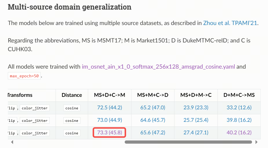
使用 Multi-source domain generalization 章节 osnet_ain_x1_0 的 MS+D+C->M 权重 osnet_ain_ms_d_c.pth.tar。
https://kaiyangzhou.github.io/deep-person-reid/MODEL_ZOO
1.3 导出 onnx
将 osnet_ain_ms_d_c.pth.tar 权重文件存放到项目根目录,编写并运行 onnx 导出脚本。
import torch
from torchreid.utils.feature_extractor import FeatureExtractordef export_onnx(model, im):f = 'osnet_ain_x1_0.onnx'torch.onnx.export(model.cpu(),im.cpu(),f,opset_version=11,do_constant_folding=True,input_names=['input'],output_names=['output'])return 0if __name__ == "__main__":extractor = FeatureExtractor(model_name="osnet_ain_x1_0",model_path="./osnet_ain_ms_d_c.pth.tar",device=str('cpu'))im = torch.zeros(1, 3, 256, 128).to('cpu')export_onnx(extractor.model.eval(), im)
1.4 检查 onnx 和 pytorch 一致性
import onnx
import torch
import onnxruntime as ort
import numpy as np
from pathlib import Path
from torchreid.utils.feature_extractor import FeatureExtractordef cosine_similarity(a, b):a = np.array(a)b = np.array(b)return np.dot(a, b) / (np.linalg.norm(a) * np.linalg.norm(b))def max_difference(a, b):a = np.array(a).ravel()b = np.array(b).ravel()diff = np.abs(a - b)max_diff = np.max(diff)max_idx = np.argmax(diff)print(f"最大差值: {max_diff},位置索引: {max_idx}")return max_diff, max_idxif __name__ == "__main__":extractor = FeatureExtractor(model_name="osnet_ain_x1_0",model_path="./osnet_ain_ms_d_c.pth.tar",device=str('cpu'))im = torch.randn(1, 3, 256, 128).to('cpu')with torch.no_grad():pt_model = extractor.model.eval()output = pt_model(im)onnx_path = 'osnet_ain_x1_0.onnx'session = ort.InferenceSession(onnx_path, providers=['CPUExecutionProvider'])input_tensor =im.numpy()input_name = session.get_inputs()[0].nameoutputs = session.run(None, {input_name: input_tensor})output_tensor = outputs[0]print(cosine_similarity(output.numpy().reshape(-1), output_tensor.reshape(-1)))max_difference(output.numpy().reshape(-1), output_tensor.reshape(-1))
如果多次运行,相似度打印均为 1,且最大差值均在 e-5 以内,则可认为 onnx 和 pytorch 的输出保持一致。
二、PTQ 量化
2.1 生成校准数据
可以从官方数据集(Market-1501-v15.09.15)中选择数百张 jpg 图片用来生成校准数据。
在生成校准数据前,需要明确预处理参数,在源码 deep-person-reid-master/torchreid/data/transforms.py 中,可以得知训练时会将图片直接 resize 成模型输入尺寸,并使用 imagenet 数据集的标准归一化参数,即:
norm_mean = [0.485, 0.456, 0.406]
norm_std = [0.229, 0.224, 0.225]
且由归一化参数可知,模型训练时使用的色彩通道顺序是 rgb。
此时可以基于 horizon_model_convert_sample 提供的脚本生成校准数据,只需基于 02_preprocess.sh 和 preprocess.py 脚本做如下改动:
python3 ../../../data_preprocess.py \--src_dir ./market_1501_jpg \    # 从Market-1501-v15.09.15数据集挑选的jpg图片--dst_dir ./calib_data_rgb_f32 \ # 生成的校准数据文件夹--pic_ext .rgb \                 # 色彩通道顺序--read_mode opencv \             # 读图方式使用opencv--saved_data_type float32 \      # 校准数据的数据类型使用float32--cal_img_num 300                # 生成300份校准数据
from horizon_tc_ui.data.transformer import (BGR2RGBTransformer, HWC2CHWTransformer, ResizeTransformer)def calibration_transformers():transformers = [ResizeTransformer(target_size=(256, 128)),  # 直接对图像做resizeHWC2CHWTransformer(),                       # 从HWC更改为CHWBGR2RGBTransformer(data_format="CHW"),      # 将色彩通道顺序更改为RGB]return transformers
由于归一化计算会集成到 PTQ 生成模型的预处理节点中,因此校准数据无需做归一化处理。
2.2 量化编译
推荐使用如下 YAML 配置:
calibration_parameters:cal_data_dir: calib_data_rgb_f32cal_data_type: float32calibration_type: maxmax_percentile: 0.99999optimization: set_all_nodes_int16run_on_cpu: "/conv1/bn/InstanceNormalization_mean1;/conv1/bn/InstanceNormalization_sub1;/conv1/bn/InstanceNormalization_mul1;/conv1/bn/InstanceNormalization_mean2;/conv1/bn/InstanceNormalization_reciprocal;/conv1/bn/InstanceNormalization_mul2;/conv1/bn/InstanceNormalization_mul3;/conv2/conv2.0/IN/InstanceNormalization_mean1;/conv2/conv2.0/IN/InstanceNormalization_sub1;/conv2/conv2.0/IN/InstanceNormalization_mul1;/conv2/conv2.0/IN/InstanceNormalization_mean2;/conv2/conv2.0/IN/InstanceNormalization_reciprocal;/conv2/conv2.0/IN/InstanceNormalization_mul2;/conv2/conv2.0/IN/InstanceNormalization_mul3"
compiler_parameters:jobs: 32optimize_level: O3
input_parameters:input_name: inputinput_shape: 1x3x256x128input_type_rt: nv12input_type_train: rgbinput_layout_train: NCHWnorm_type: 'data_mean_and_scale'mean_value: 123.675 116.28 103.53scale_value: 0.01712475383 0.0175070028 0.0174291938998
model_parameters:march: bayes-eonnx_model: osnet_ain_x1_0.onnxoutput_model_file_prefix: reidworking_dir: model_output
这里使用 nv12 作为板端模型的输入,mean_value 和 scale_value 由归一化参数计算得到。同时,考虑到 InstanceNormalization 算子的量化风险较高,因此为模型中的前两个 InstanceNormalization 配置浮点计算精度,YAML 中 run_on_cpu 配置的算子较多是因为 InstanceNormalization 会被 PTQ 拆分成多个算子。
可以使用以下命令编译:
hb_mapper makertbin --config osnet_config.yaml --model-type onnx
编译完成后,日志打印的相似度如下(quantized.onnx 对比 optimized.onnx):
=========================================================================
Output  Cosine Similarity  L1 Distance  L2 Distance  Chebyshev Distance
-------------------------------------------------------------------------
output  0.995540           0.057718     0.008716     0.482978
余弦相似度>0.99,可初步认为量化精度满足需求。
2.3 验证 PTQ 生成 onnx 的输出相似度
在编译流程结束后,可以手动验证各 PTQ 生成物和原始 onnx 的输出相似度,及时发现可能的精度问题。
*请根据不同的计算平台修改代码。
import cv2
import numpy as np
from PIL import Image
from horizon_tc_ui import HB_ONNXRuntime        def cosine_similarity(a, b):a = np.array(a)b = np.array(b)return np.dot(a, b) / (np.linalg.norm(a) * np.linalg.norm(b))def bgr2nv12(image):image = image.astype(np.uint8) height, width = image.shape[0], image.shape[1] yuv420p = cv2.cvtColor(image, cv2.COLOR_BGR2YUV_I420).reshape((height * width * 3 // 2, )) y = yuv420p[:height * width] uv_planar = yuv420p[height * width:].reshape((2, height * width // 4)) uv_packed = uv_planar.transpose((1, 0)).reshape((height * width // 2, )) nv12 = np.zeros_like(yuv420p) nv12[:height * width] = y nv12[height * width:] = uv_packed return nv12 def nv12Toyuv444(nv12, target_size): height = target_size[0] width = target_size[1] nv12_data = nv12.flatten() yuv444 = np.empty([height, width, 3], dtype=np.uint8) yuv444[:, :, 0] = nv12_data[:width * height].reshape(height, width) u = nv12_data[width * height::2].reshape(height // 2, width // 2) yuv444[:, :, 1] = Image.fromarray(u).resize((width, height),resample=0) v = nv12_data[width * height + 1::2].reshape(height // 2, width // 2) yuv444[:, :, 2] = Image.fromarray(v).resize((width, height),resample=0) return yuv444 def rgb_preprocess(img_path):bgr_input = cv2.imread(img_path)bgr_input = cv2.resize(bgr_input, (128,256), interpolation=cv2.INTER_LINEAR)rgb_input = cv2.cvtColor(bgr_input, cv2.COLOR_BGR2RGB)mean = np.array([123.675, 116.28, 103.53], dtype=np.float32)scale = np.array([0.01712475383, 0.0175070028, 0.0174291938998], dtype=np.float32)rgb_input = (rgb_input - mean) * scalergb_input = rgb_input[np.newaxis,:,:,:]rgb_input = np.transpose(rgb_input, (0, 3, 1, 2))return rgb_inputdef yuv444_preprocess(img_path):bgr_input = cv2.imread(img_path)bgr_input = cv2.resize(bgr_input, (128,256), interpolation=cv2.INTER_LINEAR)nv12_input = bgr2nv12(bgr_input)yuv444 = nv12Toyuv444(nv12_input, (256,128))yuv444_nhwc = yuv444[np.newaxis,:,:,:]yuv444_nchw = np.transpose(yuv444_nhwc, (0, 3, 1, 2))return yuv444_nhwc, yuv444_nchwdef main(): rgb_input = rgb_preprocess("test_img.jpg")yuv444_nhwc, yuv444_nchw = yuv444_preprocess("test_img.jpg")sess = HB_ONNXRuntime(model_file="./osnet_ain_x1_0.onnx")input_names = sess.input_namesoutput_names = sess.output_namesinput_info = {input_names[0]: rgb_input}onnx_output = sess.run(output_names, input_info)sess = HB_ONNXRuntime(model_file="./model_output/reid_original_float_model.onnx")input_info = {input_names[0]: yuv444_nchw}ori_output = sess.run(output_names, input_info)sess = HB_ONNXRuntime(model_file="./model_output/reid_optimized_float_model.onnx")input_info = {input_names[0]: yuv444_nchw}opt_output = sess.run(output_names, input_info)sess = HB_ONNXRuntime(model_file="./model_output/reid_calibrated_model.onnx")input_info = {input_names[0]: yuv444_nchw}calib_output = sess.run(output_names, input_info)sess = HB_ONNXRuntime(model_file="./model_output/reid_quantized_model.onnx")input_info = {input_names[0]: yuv444_nhwc}quant_output = sess.run(output_names, input_info)print("onnx_ori ", cosine_similarity(onnx_output[0].reshape(-1), ori_output[0].reshape(-1)))print("onnx_opt ", cosine_similarity(onnx_output[0].reshape(-1), opt_output[0].reshape(-1)))print("onnx_calib ", cosine_similarity(onnx_output[0].reshape(-1), calib_output[0].reshape(-1)))print("onnx_quant ", cosine_similarity(onnx_output[0].reshape(-1), quant_output[0].reshape(-1)))if __name__ == '__main__':main()
PTQ 各阶段生成的 onnx 和原始 onnx 的相似度打印结果如下:
onnx_ori  0.99779123
onnx_opt  0.9977911
onnx_calib  0.99509
onnx_quant  0.9942628
余弦相似度均>0.99,可进一步认为量化精度满足需求。
三、精度评测
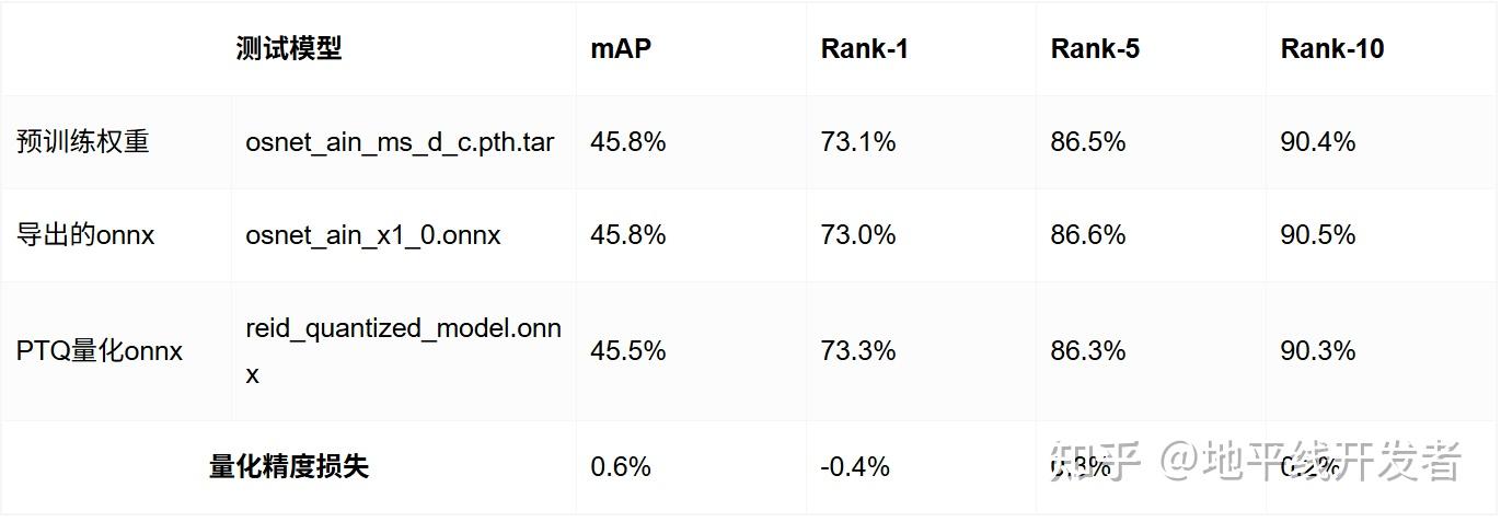
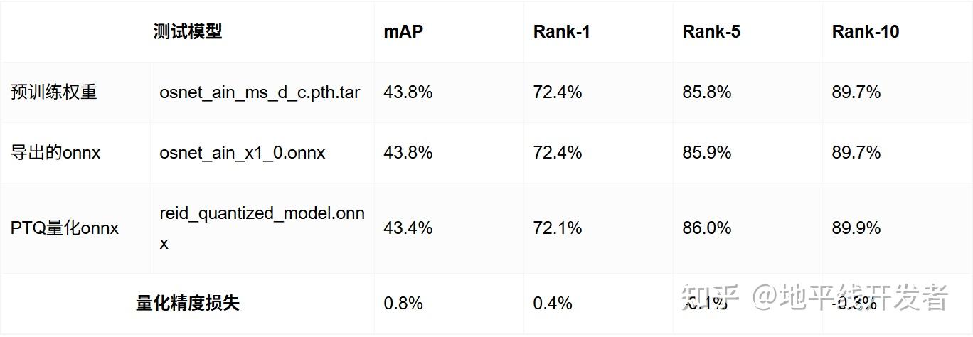
3.1 评测结果
测试数据集:Market-1501-v15.09.15
1.距离度量方式:cosine
2.距离度量方式:euclidean
3.2 评测方法
3.2.1 预训练权重
在第一章配置好的官方运行环境中,使用代码仓库的现有方法对预训练权重做精度评测。
PYTHONPATH=. python3 scripts/main.py \
--config-file configs/im_osnet_ain_x1_0_softmax_256x128_amsgrad_cosine.yaml \
--root ./ \
model.load_weights ./osnet_ain_ms_d_c.pth.tar \
test.evaluate True
3.2.2 导出的 onnx
需要基于第一章配置好的官方运行环境,额外安装 onnxruntime 和 tqdm 模块。
pip install onnxruntime
pip install tqdm
测试时,datamanager 参数需要和 configs/im_osnet_ain_x1_0_softmax_256x128_amsgrad_cosine.yaml 对齐。
import cv2
import torch
import numpy as np
import onnxruntime as ort
from PIL import Image
from tqdm import tqdmfrom torchreid.data import ImageDataManager
from torchreid.metrics import compute_distance_matrix, evaluate_rankdef extract_feature(img_path):img = cv2.imread(img_path)img = cv2.cvtColor(img, cv2.COLOR_BGR2RGB)img = Image.fromarray(img)img = transform(img)img = img.unsqueeze(0).numpy()feat = session.run(None, {input_name: img})[0]return feat[0]def extract_features(dataset):features, pids, camids = [], [], []for img_path, pid, camid, _ in tqdm(dataset, desc="Extracting features"):feat = extract_feature(img_path)features.append(feat)pids.append(pid)camids.append(camid)return np.stack(features), np.array(pids), np.array(camids)datamanager = ImageDataManager(use_gpu=False,root="./",sources=['market1501'],height=256,width=128,batch_size_train=64,batch_size_test=1,transforms=['random_flip', 'color_jitter']
)if __name__ == "__main__":query_loader = datamanager.test_loader['market1501']['query']gallery_loader = datamanager.test_loader['market1501']['gallery']query = query_loader.dataset.querygallery = gallery_loader.dataset.gallerytransform = query_loader.dataset.transformsession = ort.InferenceSession('osnet_ain_x1_0.onnx', providers=['CPUExecutionProvider'])input_name = session.get_inputs()[0].namequery_features, query_pids, query_camids = extract_features(query)gallery_features, gallery_pids, gallery_camids = extract_features(gallery)distmat = compute_distance_matrix(torch.tensor(query_features),torch.tensor(gallery_features),metric='cosine').numpy()cmc, mAP = evaluate_rank(distmat, query_pids, gallery_pids, query_camids, gallery_camids, use_cython=False)print("\n=== Market1501 Evaluation Results (ONNX model) ===")print(f"mAP     : {mAP:.2%}")print(f"Rank-1  : {cmc[0]:.2%}")print(f"Rank-5  : {cmc[4]:.2%}")print(f"Rank-10 : {cmc[9]:.2%}")
3.2.3 PTQ 量化 onnx
需要基于第一章配置好的官方运行环境,额外安装 onnxruntime 和 tqdm 模块,并安装 horizon-nn/hmct 和 horizon-tc-ui。
pip install onnxruntime
pip install tqdm
pip install horizon_nn-1.1.0.post0.dev202506060002+840a0a685d053923c1a577c5032b7e0cfc84e6ac-cp310-cp310-linux_x86_64.whl --no-deps
pip install horizon_tc_ui-1.24.4-cp310-cp310-linux_x86_64.whl --no-deps
测试时,datamanager 参数需要和 configs/im_osnet_ain_x1_0_softmax_256x128_amsgrad_cosine.yaml 对齐,且需要把输入数据处理成 yuv444 类型。
import cv2
import torch
import numpy as np
from PIL import Image
from tqdm import tqdm
from horizon_tc_ui import HB_ONNXRuntimefrom torchreid.data import ImageDataManager
from torchreid.metrics import compute_distance_matrix, evaluate_rankdef bgr2nv12(image):image = image.astype(np.uint8) height, width = image.shape[0], image.shape[1] yuv420p = cv2.cvtColor(image, cv2.COLOR_BGR2YUV_I420).reshape((height * width * 3 // 2, )) y = yuv420p[:height * width] uv_planar = yuv420p[height * width:].reshape((2, height * width // 4)) uv_packed = uv_planar.transpose((1, 0)).reshape((height * width // 2, )) nv12 = np.zeros_like(yuv420p) nv12[:height * width] = y nv12[height * width:] = uv_packed return nv12 def nv12Toyuv444(nv12, target_size): height = target_size[0] width = target_size[1] nv12_data = nv12.flatten() yuv444 = np.empty([height, width, 3], dtype=np.uint8) yuv444[:, :, 0] = nv12_data[:width * height].reshape(height, width) u = nv12_data[width * height::2].reshape(height // 2, width // 2) yuv444[:, :, 1] = Image.fromarray(u).resize((width, height),resample=0) v = nv12_data[width * height + 1::2].reshape(height // 2, width // 2) yuv444[:, :, 2] = Image.fromarray(v).resize((width, height),resample=0) return yuv444 def preprocess_nhwc(img_path):bgr_input = cv2.imread(img_path)bgr_input = cv2.resize(bgr_input, (128,256), interpolation=cv2.INTER_LINEAR)nv12_input = bgr2nv12(bgr_input)yuv444 = nv12Toyuv444(nv12_input, (256,128))yuv444 = yuv444[np.newaxis,:,:,:]return yuv444def extract_feature(img_path):for input_name in input_names:feed_dict[input_name] = preprocess_nhwc(img_path)feat = sess.run(output_names, feed_dict)return feat[0]def extract_features(dataset):features, pids, camids = [], [], []for img_path, pid, camid, _ in tqdm(dataset, desc="Extracting features"):feat = extract_feature(img_path)features.append(feat)pids.append(pid)camids.append(camid)return np.stack(features), np.array(pids), np.array(camids)if __name__ == "__main__":datamanager = ImageDataManager(use_gpu=False,root="./",sources=['market1501'],height=256,width=128,batch_size_train=64,batch_size_test=1,transforms=['random_flip', 'color_jitter'])query_loader = datamanager.test_loader['market1501']['query']gallery_loader = datamanager.test_loader['market1501']['gallery']query = query_loader.dataset.querygallery = gallery_loader.dataset.gallerytransform = query_loader.dataset.transformsess = HB_ONNXRuntime(model_file='./model_output_inx2_cpu/reid_quantized_model.onnx')input_names = [input.name for input in sess.get_inputs()]output_names = [output.name for output in sess.get_outputs()]feed_dict = dict()query_features, query_pids, query_camids = extract_features(query)gallery_features, gallery_pids, gallery_camids = extract_features(gallery)distmat = compute_distance_matrix(torch.tensor(query_features.squeeze(1)),torch.tensor(gallery_features.squeeze(1)),metric='cosine').numpy()cmc, mAP = evaluate_rank(distmat, query_pids, gallery_pids, query_camids, gallery_camids, use_cython=False)print("\n=== Market1501 Evaluation Results (ONNX model) ===")print(f"mAP     : {mAP:.2%}")print(f"Rank-1  : {cmc[0]:.2%}")print(f"Rank-5  : {cmc[4]:.2%}")print(f"Rank-10 : {cmc[9]:.2%}")
四、性能评测
4.1 评测结果
Running condition:Thread number is: 1Frame count   is: 1000Program run time: 51433.128000 ms
Perf result:Frame totally latency is: 51417.804688 msAverage    latency    is: 51.417805 msFrame      rate       is: 19.442722 FPS
以 X5 为例,该模型的单线程推理延时为 51.4ms,对应 FPS 为 19.4
Latency 是指单流程推理模型所耗费的平均时间,重在表示在资源充足的情况下推理一帧的平均耗时,体现在上板运行是单核单线程统计。
FPS 是指多流程同时进行模型推理平均一秒推理的帧数,重在表示充分使用资源情况下模型的吞吐,体现在上板运行为单核多线程;统计方法是同时起多个线程进行模型推理,计算平均 1s 推理的总帧数。
Latency 与 FPS 的统计情景不同,Latency 为单流程(单核单线程)推理,FPS 为多流程(单核多线程)推理,因此推算不一致;若统计 FPS 时将流程(线程)数量设置为 1 ,则通过 Latency 推算 FPS 和测出的一致。
4.2 评测方法
可板端使用 hrt_model_exec 工具获取模型的实测性能数据,测试命令如下:
hrt_model_exec perf --model-file reid.bin --frame-count 1000 --thread-num 1
417.804688 msAverage    latency    is: 51.417805 msFrame      rate       is: 19.442722 FPS