连续概率分布 (拉普拉斯分布)
一、说明
类似于高斯分布,还有其他的对称负指数分布,比如柯西分布,拉普拉斯分布,本篇讲述拉普拉斯分布。
二、基本概念
在概率论和统计学中,拉普拉斯分布是一种连续概率分布,以皮埃尔-西蒙·拉普拉斯的名字命名。它有时也称为双指数分布,因为它可以被认为是两个指数分布背靠背沿 x 轴拼接在一起。
2.1 密度函数
随机变量具有拉普拉斯 laplace ( μ , b ) {\displaystyle \operatorname {laplace} (\mu ,b)} laplace(μ,b)分布,如果其概率密度函数pdf为

在这里
- μ {\displaystyle \mu} μ是位置参数.用于确定分布的中心
- 并且 b > 0 {\displaystyle b>0} b>0,用于控制分布的散布或宽度,有时被称为“多样性”,是一个尺度参数。
如果 μ = 0 {\displaystyle \mu =0} μ=0和 b = 1 {\displaystyle b=1} b=1,正半线恰好是按 1/2 缩放的指数分布。
2.2 分布函数
由于使用了绝对值函数,拉普拉斯分布很容易积分(如果区分两种对称情况) 。其累积分布函数如下:

三、Python 中的示例
- 具有不同μ的拉普拉斯分布
下面的第一个代码是一个 Python 脚本,它说明了具有不同 μ 值(位置参数)的拉普拉斯分布。
import numpy as np
import matplotlib.pyplot as plt# Define the Laplacian distribution function
def laplacian_pdf(x, mu, b):return (1 / (2 * b)) * np.exp(-np.abs(x - mu) / b)# Values of the location parameter 'mu'
mu_values = [-2, 0, 2]
b = 1  # Fixed scale parameter# Create a range of x values
x = np.linspace(-10, 10, 1000)# Plot the Laplacian distributions for varying mu
plt.figure(figsize=(12, 6))for mu in mu_values:y = laplacian_pdf(x, mu, b)plt.plot(x, y, label=f'μ = {mu}')plt.title('Laplacian Distribution with Varying μ')
plt.xlabel('x')
plt.ylabel('Probability Density')
plt.legend()
plt.grid(True)
plt.show()
这是上述代码的输出:
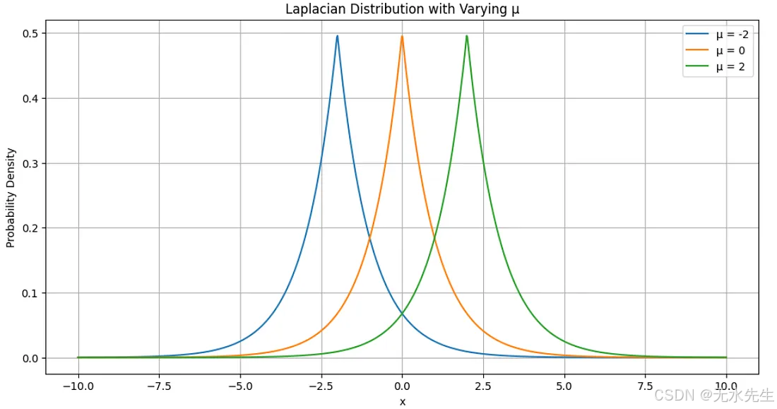
- 此脚本绘制位置参数 μ 不同值的拉普拉斯分布,其中具有固定尺度参数 b=1。
- 该函数计算 中每个 μ 值的概率密度laplacian_pdf。
- 具有变化 b 的拉普拉斯分布
下面的第二段代码是一个 Python 脚本,它说明了具有不同 b (scale 参数)值的拉普拉斯分布。
import numpy as np
import matplotlib.pyplot as plt# Define the Laplacian distribution function
def laplacian_pdf(x, mu, b):return (1 / (2 * b)) * np.exp(-np.abs(x - mu) / b)# Values of the scale parameter 'b'
b_values = [0.5, 1, 2]
mu = 0  # Fixed location parameter# Create a range of x values
x = np.linspace(-10, 10, 1000)# Plot the Laplacian distributions for varying b
plt.figure(figsize=(12, 6))for b in b_values:y = laplacian_pdf(x, mu, b)plt.plot(x, y, label=f'b = {b}, σ = {np.sqrt(2)*b:.2f}')plt.title('Laplacian Distribution with Varying b')
plt.xlabel('x')
plt.ylabel('Probability Density')
plt.legend()
plt.grid(True)
plt.show()
这是上述代码的输出:
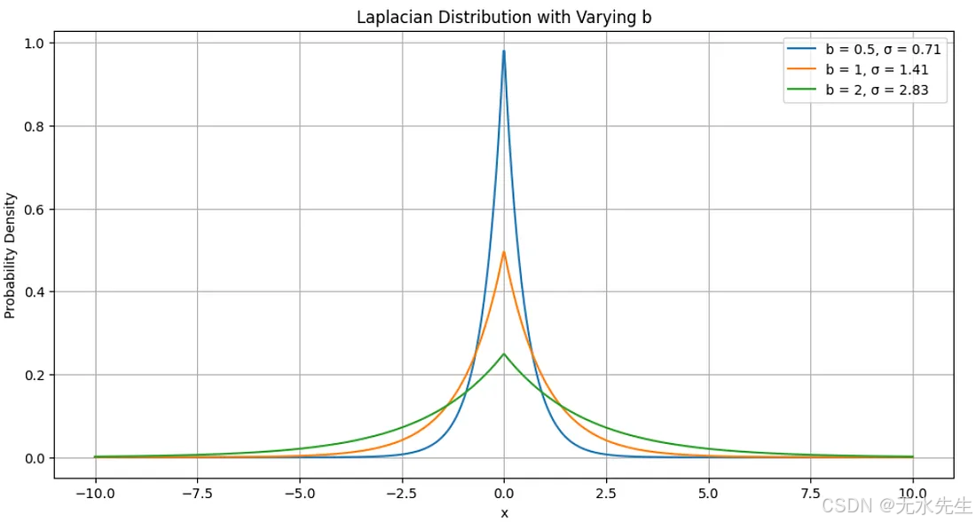
- 此脚本绘制刻度参数 b 的不同值的拉普拉斯分布,固定位置参数 μ = 0
- 该函数计算laplacian_pdf中每个 b 值的概率密度b_values
四、问题:为什么拉普拉斯分布具有尖锐的峰值和沉重的尾部?
拉普拉斯分布具有尖锐的峰值和沉重的尾部,因为它的概率密度函数随着与平均值的绝对距离呈指数下降,导致与多项式衰减的分布(例如正态分布)相比,尾部的衰减速度较慢。