目标框的位置以及大小的分布

目标框的位置以及大小的分布

方法步骤：

数据集统一化：
和yolo训练和推理的预处理一样，等比例缩放 + 边缘填充，换算标签值。

中心点分布：

• 按 8×8 网格（每格 80×80像素）统计每个网格的目标数及占比（占比 = 网格数 / 总目标数）；
• 分别打印出两个8乘8的矩阵，目标数的和目标数占比的。
• 用占比的值绘制热力图，热力图可视化，标注占比（<1% 时特殊显示），保留两位小数。

框大小分布：

• 计算 640×640 中的归一化面积（(w_640/640)×(h_640/640)），绘制直方图（等频分箱，10~20 箱）；
• 计算 640×640 中的归一化对角线长度（√((w_640/640)² + (h_640/640)² )），绘制直方图（同前分箱方式）。
• 两个图都是横坐标从0到最大值等分为10份（变量记录方便修改）
• 打印出两个的各个统计量（均值，方差，中位数等等）

分析结果说明

两数据集参与统计的样本情况

testB-3000，DUT-Anti-UAV-train
参数相同：

    sampling_step=1,       # 步长grid_size=8,           # 8×8网格bin_num=10,            # 直方图分箱数save_plots='./DUT_plot',   # 保存图片到plot目录，False表示不保存仅显示hist_xlim=[0, 0.03]     # 直方图横坐标范围，这里设置为0到0.2

testB的数据集信息：原始样本数：3000原始样本中的目标数量：3719抽样后样本数：3000抽样后的目标数量：3719抽样步长：1图像文件夹：C:\baidunetdiskdownload\testB3000-new\images标签文件夹：C:\baidunetdiskdownload\testB3000-new\labels
处理完成：总目标数：3719DUT的数据集信息：原始样本数：5197原始样本中的目标数量：5243抽样后样本数：5197抽样后的目标数量：5243抽样步长：1图像文件夹：/mnt/Virgil/YOLO/drone_dataset/DUT-Anti-UAV-train/images标签文件夹：/mnt/Virgil/YOLO/drone_dataset/DUT-Anti-UAV-train/labels
处理完成：总目标数：5243

目标位置分布对比

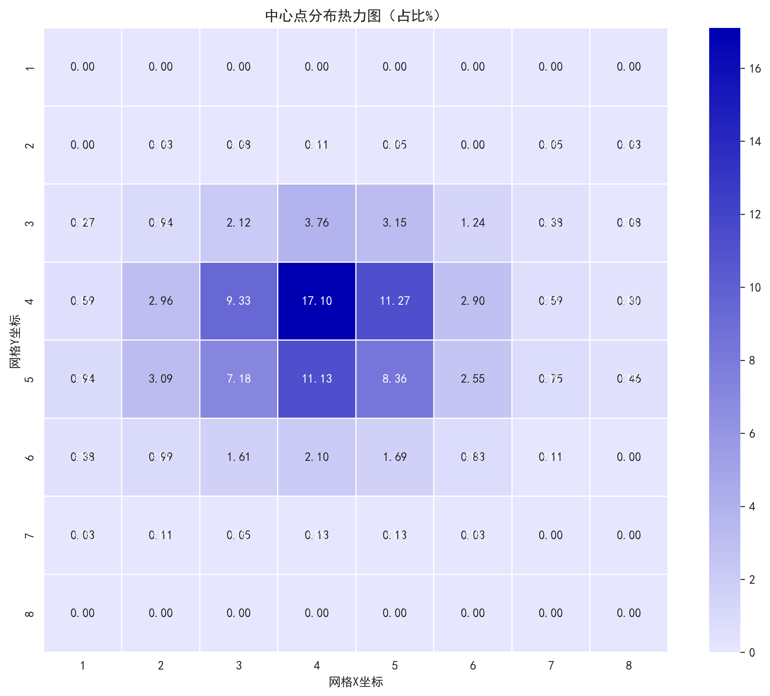
testB:

DUT

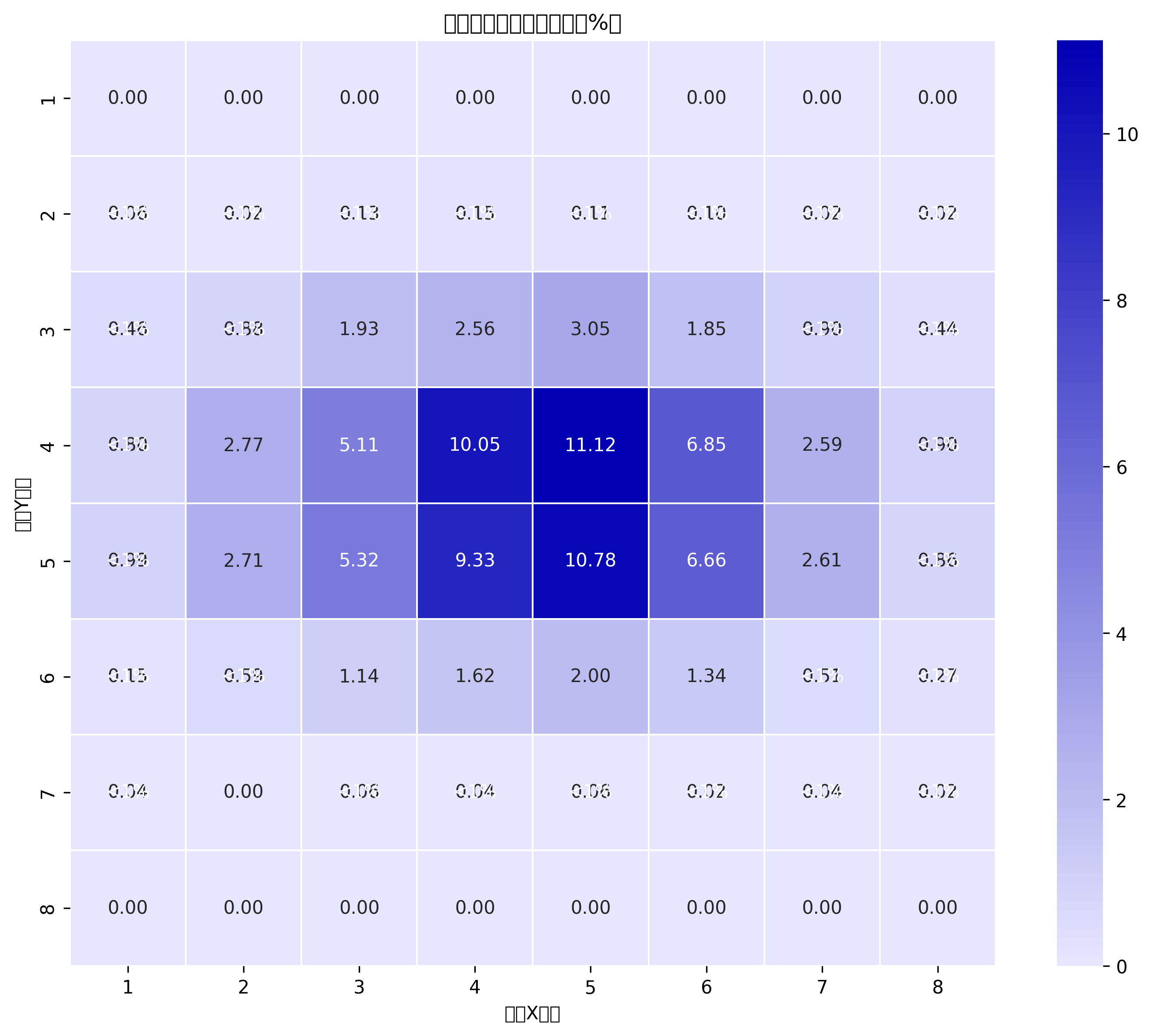
都集中在中心，并且上下边缘都没有目标。testB的可能因为数据量少中心有些偏左上角。

具体目标数矩阵：

中心点分布矩阵（目标数）：
testB：
[[  0   0   0   0   0   0   0   0][  0   1   3   4   2   0   2   1][ 10  35  79 140 117  46  14   3][ 22 110 347 636 419 108  22  11][ 35 115 267 414 311  95  28  17][ 14  37  60  78  63  31   4   0][  1   4   2   5   5   1   0   0][  0   0   0   0   0   0   0   0]]DUT：
[[  0   0   0   0   0   0   0   0][  3   1   7   8   6   5   1   1][ 24  46 101 134 160  97  47  23][ 42 145 268 527 583 359 136  47][ 52 142 279 489 565 349 137  45][  8  31  60  85 105  70  27  14][  2   0   3   2   3   1   2   1][  0   0   0   0   0   0   0   0]]

目标框大小分布对比[0, 0.03]

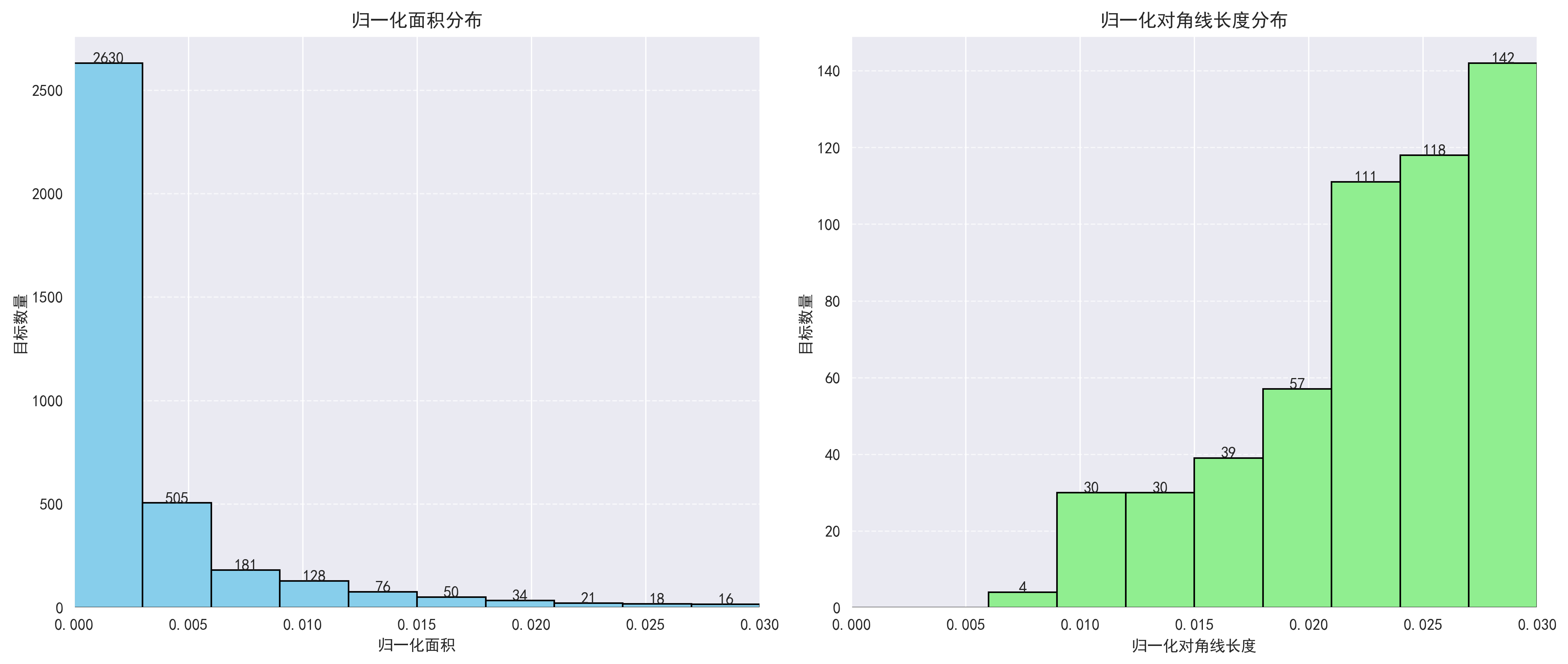
testB

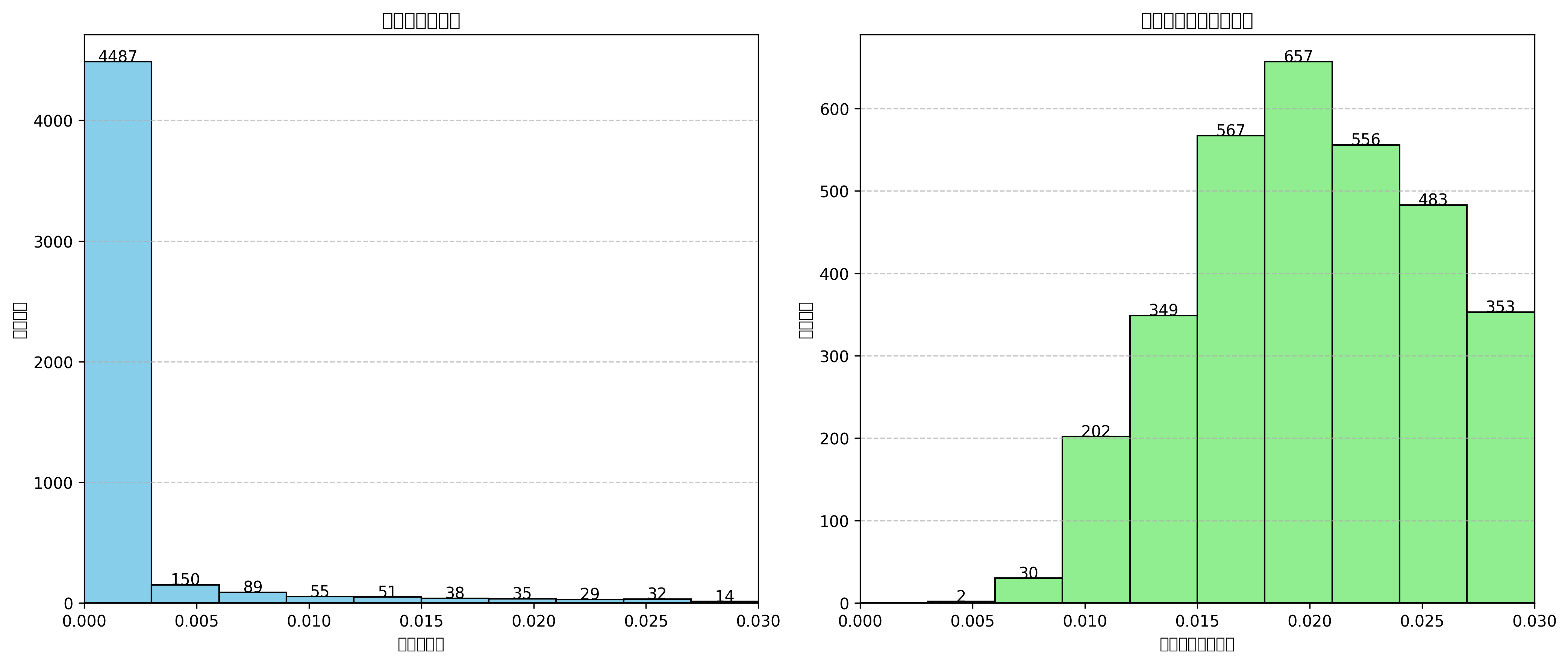
DUT

详细统计信息

testB
框面积统计量：均值：0.003754方差：0.000057中位数：0.001302最小值：0.000027最大值：0.194579框对角线统计量：均值：0.079778方差：0.003986中位数：0.059560最小值：0.008240最大值：0.730294DUT
框面积统计量：均值：0.007510方差：0.001106中位数：0.000265最小值：0.000011最大值：0.528570框对角线统计量：均值：0.063983方差：0.013848中位数：0.025542最小值：0.004914最大值：1.049200

代码

import os
import random
import numpy as np
import matplotlib.pyplot as plt
from matplotlib.colors import LinearSegmentedColormap
from PIL import Image
import seaborn as sns# 设置中文显示
plt.rcParams["font.family"] = ["SimHei", "WenQuanYi Micro Hei", "Heiti TC"]
plt.rcParams['axes.unicode_minus'] = False  # 解决负号显示问题class YOLODatasetAnalyzer:def __init__(self, image_dir, label_dir, sampling_step=1, grid_size=8, bin_num=10, save_plots=False, hist_xlim=None):"""初始化YOLO数据集分析器Args:image_dir: 图像文件夹路径label_dir: 标签文件夹路径sampling_step: 抽样步长，例如每4个样本取1个grid_size: 中心点分布热力图的网格大小bin_num: 直方图的分箱数量save_plots: 是否保存可视化图片，False表示不保存仅显示，字符串表示保存目录hist_xlim: 直方图横坐标范围，格式为[min, max]，None表示自动适应"""self.image_dir = image_dirself.label_dir = label_dirself.sampling_step = sampling_stepself.grid_size = grid_sizeself.bin_num = bin_numself.save_plots = save_plotsself.hist_xlim = hist_xlim if hist_xlim is not None else [0, None]  # 默认为0到最大值self.image_files = []self.label_files = []self.sample_image_files = []self.sample_label_files = []self.total_objects = 0self.sample_total_objects = 0self.center_distribution = np.zeros((grid_size, grid_size), dtype=int)self.box_areas = []self.box_diagonals = []def prepare_dataset(self):"""准备数据集，获取图像和标签文件列表并进行抽样"""# 获取所有图像和标签文件original_total_objects = 0for file in os.listdir(self.image_dir):if file.lower().endswith(('.png', '.jpg', '.jpeg')):image_path = os.path.join(self.image_dir, file)label_file = os.path.splitext(file)[0] + '.txt'label_path = os.path.join(self.label_dir, label_file)# 检查标签文件是否存在if os.path.exists(label_path):# 计算该标签文件中的目标数量with open(label_path, 'r') as f:lines = f.readlines()object_count = len(lines)original_total_objects += object_countself.image_files.append(image_path)self.label_files.append(label_path)# 随机分层抽样if self.sampling_step > 1:indices = list(range(0, len(self.image_files), self.sampling_step))random.shuffle(indices)self.sample_image_files = [self.image_files[i] for i in indices]self.sample_label_files = [self.label_files[i] for i in indices]else:self.sample_image_files = self.image_filesself.sample_label_files = self.label_files# 计算抽样后的目标数量for label_file in self.sample_label_files:with open(label_file, 'r') as f:self.sample_total_objects += len(f.readlines())print(f"数据集信息：")print(f"  原始样本数：{len(self.image_files)}")print(f"  原始样本中的目标数量：{original_total_objects}")print(f"  抽样后样本数：{len(self.sample_image_files)}")print(f"  抽样后的目标数量：{self.sample_total_objects}")print(f"  抽样步长：{self.sampling_step}")print(f"  图像文件夹：{self.image_dir}")print(f"  标签文件夹：{self.label_dir}")# 创建保存图片的目录if isinstance(self.save_plots, str):os.makedirs(self.save_plots, exist_ok=True)def process_labels(self):"""处理标签，计算中心点分布和框大小"""for image_file, label_file in zip(self.sample_image_files, self.sample_label_files):# 获取图像尺寸try:img = Image.open(image_file)img_width, img_height = img.sizeexcept Exception as e:print(f"无法读取图像 {image_file}: {e}")continue# 读取标签with open(label_file, 'r') as f:lines = f.readlines()for line in lines:parts = line.strip().split()if len(parts) < 5:  # 确保标签格式正确continue# 解析标签class_id = int(parts[0])x_center_norm = float(parts[1])y_center_norm = float(parts[2])width_norm = float(parts[3])height_norm = float(parts[4])# 计算预处理后的坐标（等比例缩放+填充到640×640）scale = min(640/img_width, 640/img_height)new_width = img_width * scalenew_height = img_height * scalepad_w = (640 - new_width) / 2pad_h = (640 - new_height) / 2# 转换为640×640图像中的像素坐标x_center_640 = x_center_norm * img_width * scale + pad_wy_center_640 = y_center_norm * img_height * scale + pad_hwidth_640 = width_norm * img_width * scaleheight_640 = height_norm * img_height * scale# 更新中心点分布grid_x = int(x_center_640 // (640 / self.grid_size))grid_y = int(y_center_640 // (640 / self.grid_size))grid_x = min(grid_x, self.grid_size - 1)  # 防止越界grid_y = min(grid_y, self.grid_size - 1)self.center_distribution[grid_y, grid_x] += 1  # 注意matplotlib中y轴向下self.total_objects += 1# 计算归一化面积和对角线长度norm_width = width_640 / 640norm_height = height_640 / 640area = norm_width * norm_heightdiagonal = np.sqrt(norm_width**2 + norm_height**2)self.box_areas.append(area)self.box_diagonals.append(diagonal)print(f"处理完成：")print(f"  总目标数：{self.total_objects}")def analyze_center_distribution(self):"""分析中心点分布并可视化"""if self.total_objects == 0:print("没有可分析的目标")return# 计算占比center_percentage = self.center_distribution / self.total_objects * 100# 打印矩阵print("\n中心点分布矩阵（目标数）：")print(self.center_distribution)print("\n中心点分布矩阵（占比%）：")print(np.round(center_percentage, 2))# 创建自定义颜色映射colors = [(0.9, 0.9, 1), (0, 0, 0.7)]  # 从浅蓝色到深蓝色cmap = LinearSegmentedColormap.from_list('BlueCustom', colors, N=100)# 绘制热力图plt.figure(figsize=(10, 8))ax = sns.heatmap(center_percentage, annot=True, fmt='.2f', cmap=cmap, cbar=True, square=True, linewidths=.5, xticklabels=range(1, self.grid_size+1), yticklabels=range(1, self.grid_size+1))# 处理<1%的情况for i in range(self.grid_size):for j in range(self.grid_size):if center_percentage[i, j] < 1 and center_percentage[i, j] > 0:ax.text(j+0.5, i+0.5, '<1%', ha='center', va='center', color='white')plt.title('中心点分布热力图（占比%）')plt.xlabel('网格X坐标')plt.ylabel('网格Y坐标')plt.tight_layout()# 保存图片if isinstance(self.save_plots, str):save_path = os.path.join(self.save_plots, 'center_distribution_heatmap.png')plt.savefig(save_path, dpi=300, bbox_inches='tight')# 显示图片plt.show()def analyze_box_size(self):"""分析框大小并可视化"""if not self.box_areas:print("没有可分析的框")return# 计算统计量area_stats = {'均值': np.mean(self.box_areas),'方差': np.var(self.box_areas),'中位数': np.median(self.box_areas),'最小值': np.min(self.box_areas),'最大值': np.max(self.box_areas)}diagonal_stats = {'均值': np.mean(self.box_diagonals),'方差': np.var(self.box_diagonals),'中位数': np.median(self.box_diagonals),'最小值': np.min(self.box_diagonals),'最大值': np.max(self.box_diagonals)}# 打印统计量print("\n框面积统计量：")for key, value in area_stats.items():print(f"  {key}：{value:.6f}")print("\n框对角线统计量：")for key, value in diagonal_stats.items():print(f"  {key}：{value:.6f}")# 确定直方图横坐标范围area_min, area_max = self.hist_xlim[0], self.hist_xlim[1] or max(self.box_areas)diag_min, diag_max = self.hist_xlim[0], self.hist_xlim[1] or max(self.box_diagonals)# 绘制直方图fig, (ax1, ax2) = plt.subplots(1, 2, figsize=(14, 6))# 面积直方图_, bins, _ = ax1.hist(self.box_areas, bins=self.bin_num, range=(area_min, area_max),color='skyblue', edgecolor='black')ax1.set_title('归一化面积分布')ax1.set_xlabel('归一化面积')ax1.set_ylabel('目标数量')ax1.set_xlim(area_min, area_max)ax1.grid(axis='y', linestyle='--', alpha=0.7)# 添加数据标签for i in range(len(bins)-1):count = sum(1 for x in self.box_areas if bins[i] <= x < bins[i+1])if count > 0:ax1.text((bins[i] + bins[i+1])/2, count + max(self.box_areas)/50, f'{count}', ha='center')# 对角线直方图_, bins, _ = ax2.hist(self.box_diagonals, bins=self.bin_num, range=(diag_min, diag_max),color='lightgreen', edgecolor='black')ax2.set_title('归一化对角线长度分布')ax2.set_xlabel('归一化对角线长度')ax2.set_ylabel('目标数量')ax2.set_xlim(diag_min, diag_max)ax2.grid(axis='y', linestyle='--', alpha=0.7)# 添加数据标签for i in range(len(bins)-1):count = sum(1 for x in self.box_diagonals if bins[i] <= x < bins[i+1])if count > 0:ax2.text((bins[i] + bins[i+1])/2, count + max(self.box_diagonals)/50, f'{count}', ha='center')plt.tight_layout()# 保存图片if isinstance(self.save_plots, str):save_path = os.path.join(self.save_plots, 'box_size_distribution.png')plt.savefig(save_path, dpi=300, bbox_inches='tight')# 显示图片plt.show()def main():# 数据集路径（注意使用原始字符串或转义反斜杠）image_dir = r"C:\baidunetdiskdownload\testB3000-new\images"label_dir = r"C:\baidunetdiskdownload\testB3000-new\labels"# 创建分析器实例analyzer = YOLODatasetAnalyzer(image_dir=image_dir,label_dir=label_dir,sampling_step=1,       # 步长grid_size=8,           # 8×8网格bin_num=10,            # 直方图分箱数save_plots='./plot',   # 保存图片到plot目录，False表示不保存仅显示hist_xlim=[0, 0.03]     # 直方图横坐标范围，这里设置为0到0.2)# 执行分析analyzer.prepare_dataset()analyzer.process_labels()analyzer.analyze_center_distribution()analyzer.analyze_box_size()if __name__ == "__main__":main()