PINNs案例——二维磁场计算
基于物理信息的神经网络是一种解决偏微分方程计算问题的全新方法…
有关PINN基础详见:PINNs案例——中心热源温度场预测问题的torch代码
今日分享代码案例:二维带电流源磁场计算
该案例参考学习论文:
[1]张宇娇,孙宏达,赵志涛,徐斌,黄雄峰.基于物理信息神经网络的电磁场计算方法[J/OL].电工技术学报.
结果前瞻
问题场景
- ** 求解域** 案例选取边长为 10 的正方形区域作为研究对象,即定义域为
Ω = [ 0 , 10 ] × [ 0 , 10 ] \Omega = [0, 10] \times [0, 10] Ω=[0,10]×[0,10]。以正方形左下角为原点,正方形区域内包含一个带电流密度为1的导体,导体区域为 Ω = [ 4 , 2 ] × [ 6 , 8 ] \Omega = [4, 2] \times [6, 8] Ω=[4,2]×[6,8]。 - **参数设定:**导体处 J = 1 J = 1 J=1,导体材料为铜(copper),其余区域为空气(air),磁导率 γ \gamma γ 均为1
- **边界条件:**方形四周边界的矢量磁位为0(理想导体边界)
- **求解量:**区域内二维稳态磁场分布(矢量)
PINNs理论求解
在本案例中,我们引入矢量磁位 $ \mathbf{A} $ 来辅助磁场的计算。矢量磁位A设定为:
B = ∇ × A \mathbf{B} = \nabla \times \mathbf{A} B=∇×A
其中, B \mathbf{B} B 表示磁场强度,该关系表明磁场是矢量磁位的旋度。
在该正方形区域内,矢量磁位 $ A_z(x, y) $ 满足麦克斯韦方程,引入矢量磁位A后在二维稳态下,其数学表达式为:
( ∂ 2 A z ∂ x 2 + ∂ 2 A z ∂ y 2 ) = − μ J z \left( \frac{\partial^2 A_z}{\partial x^2} + \frac{\partial^2 A_z}{\partial y^2} \right) =-\mu J_z (∂x2∂2Az+∂y2∂2Az)=−μJz
其中:
μ \mu μ 为材料的磁导率,表示材料对磁场的响应能力;
J z J_z Jz 为电流密度在 z z z 方向的分量,表示单位面积内电流的大小;
A z ( x , y ) A_z(x, y) Az(x,y) 为矢量磁位在 z z z 方向的分量,通常用于描述二维平面内的磁场分布。
这种方程形式常见于静电学或静磁学中的泊松方程,用于描述在存在源(如电荷或电流)的情况下,势函数(如矢量磁位)的空间分布。矢量磁位的引入使得磁场的计算更为简便,尤其是在处理对称性问题或边界条件时。
本次案例中,由于存在铜导体区域(有源)和空气域(无源),故采用PINNs案例——多介质分区热传导中相同的分区思想。此处不过多介绍
损失函数可以表示为:
- PDE 残差项: 控制方程如下:
Loss PDE = 1 N c ∑ i = 1 N c ∣ f ( x c i , y c i ) ∣ 2 \text{Loss}_{\text{PDE}} = \frac{1}{N_c} \sum_{i=1}^{N_c} \left| f\left( x_c^i, y_c^i \right) \right|^2 LossPDE=Nc1i=1∑Nc f(xci,yci) 2
f ( x c i , y c i ) = ( ∂ 2 A z ∂ x 2 + ∂ 2 A z ∂ y 2 ) + μ J z f\left( x_c^i, y_c^i \right) = \left( \frac{\partial^2 A_z}{\partial x^2} + \frac{\partial^2 A_z}{\partial y^2} \right) +\mu J_z f(xci,yci)=(∂x2∂2Az+∂y2∂2Az)+μJz
注意: 由于PDE损失中需加入 μ 0 \mu_{0} μ0,而 μ 0 = 4 π ∗ 10 − 7 \mu_{0} = 4\pi * 10^{-7} μ0=4π∗10−7 数量级过小,会对神经网络的训练带来较大困难。故需对PDE方程进行简单的无量纲化操作,令 A ′ = A / μ 0 A' = A/\mu_0 A′=A/μ0, 于是可以得到 f ( x c i , y c i ) = ( ∂ 2 A z ′ ∂ x 2 + ∂ 2 A z ′ ∂ y 2 ) + μ r J z f\left( x_c^i, y_c^i \right) = \left( \frac{\partial^2 A_z'}{\partial x^2} + \frac{\partial^2 A_z'}{\partial y^2} \right) +\mu_r J_z f(xci,yci)=(∂x2∂2Az′+∂y2∂2Az′)+μrJz.预测后再将A乘 μ 0 \mu_0 μ0以还原A
- 边界条件项:在多介质问题中,边界条件除矢量磁位A=0的方形边界条件,还要添加不同介质交界面的连续性边界条件。
-
固定温度边界:
Loss BC = 1 N b ∑ i = 1 N b ∣ A ( x b i , y b i ) ∣ 2 \text{Loss}_{\text{BC}} = \frac{1}{N_b} \sum_{i=1}^{N_b} \left|A\left( x_b^i, y_b^i \right) \right|^2 LossBC=Nb1i=1∑Nb A(xbi,ybi) 2 -
介质交界面:
此案例中以A的第一类和第二类边界条件作为介质交界面的连续性条件
第一类边界条件:
Loss I1 = 1 N I ∑ j = 1 N I ∣ A p ( x I j ) − A p + 1 ( x I j ) ∣ 2 \text{Loss}_{\text{I1}} = \frac{1}{N_{I}}\sum_{j=1}^{N_{I}}\left| A_{p}\left(x_{I}^{j}\right)-A_{p+1}\left(x_{I}^{j}\right)\right|^{2} LossI1=NI1j=1∑NI Ap(xIj)−Ap+1(xIj) 2
第二类边界条件(不同介质在边界面上矢量磁位法向导数与磁导率的乘积连续):
Loss I2 = 1 N I ∑ j = 1 N I ∣ γ p ∂ A p ( x I j ) ∂ n − γ p + 1 ∂ A p + 1 ( x I j ) ∂ n ∣ 2 \text{Loss}_{\text{I2}} = \frac{1}{N_{I}}\sum_{j=1}^{N_{I}}\left|\gamma_{p}\frac{\partial A_{p}\left(x_{I}^{j}\right)}{\partial n}-\gamma_{p+1}\frac{\partial A_{p+1}\left(x_{I}^{j}\right)}{\partial n}\right|^{2} LossI2=NI1j=1∑NI γp∂n∂Ap(xIj)−γp+1∂n∂Ap+1(xIj) 2
其中:
- N I N_I NI 表示介质边界点的点数
- A p A_p Ap 表示第P个介质的矢量磁位
- γ p \gamma_ {p} γp 表示第P个介质的热导率
训练
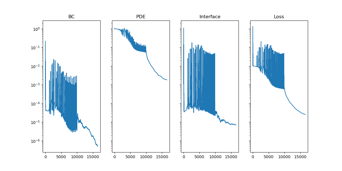
采用10000次adam优化与lbfgs优化器进行优化。各项损失收敛过程如下,收敛效果良好:
复现结果
comsol仿真结果
可见结果吻合良好
pytorch代码
为避免繁杂的点生成,作者编写了一组点生成函数,使用时单独建立points_generator.py,并在训练代码中引入。
points_generator.py
import numpy as np
from pyDOE import lhsdef generate_boundary_points(x_min, y_min, x_max, y_max, n):# 计算每条边上的点数num_points_x = int((x_max - x_min) * n) + 1num_points_y = int((y_max - y_min) * n) + 1# 生成每条边上的点bottom_edge = np.array([np.linspace(x_min, x_max, num_points_x), np.full(num_points_x, y_min)]).Ttop_edge = np.array([np.linspace(x_min, x_max, num_points_x), np.full(num_points_x, y_max)]).Tleft_edge = np.array([np.full(num_points_y, x_min), np.linspace(y_min, y_max, num_points_y)]).Tright_edge = np.array([np.full(num_points_y, x_max), np.linspace(y_min, y_max, num_points_y)]).T# 合并所有边上的点,去掉重复的角点boundary_points = np.concatenate([bottom_edge, top_edge[1:], left_edge[1:-1], right_edge[1:-1]])boundary_vertical = np.concatenate([left_edge[1:-1], right_edge[1:-1]])boundary_horizontal = np.concatenate([bottom_edge, top_edge[1:]])return boundary_points,boundary_vertical,boundary_horizontaldef generate_internal_points(x_min, y_min, x_max, y_max, n):# 计算内部点的网格x = np.linspace(x_min, x_max, int((x_max - x_min) * n) + 1)y = np.linspace(y_min, y_max, int((y_max - y_min) * n) + 1)x_grid, y_grid = np.meshgrid(x, y)# 去掉边界点x_grid = x_grid[1:-1, 1:-1]y_grid = y_grid[1:-1, 1:-1]# 将网格点转换为一维数组internal_points = np.array([x_grid.flatten(), y_grid.flatten()]).Treturn internal_pointsdef generate_mask(points, x_min, y_min, x_max, y_max):# 检查每个点是否在矩形区域内mask = (points[:, 0] >= x_min) & (points[:, 0] <= x_max) & (points[:, 1] >= y_min) & (points[:, 1] <= y_max)return maskdef lhs_internal_points(x_min, y_min, x_max, y_max, n):  '''使用超拉丁立方采样矩形区域内的点'''ub = np.array([x_max, y_max])lb = np.array([x_min, y_min])internal_points = lb + (ub - lb) * lhs(2, n)return internal_points
训练代码
import numpy as np
import matplotlib.pyplot as plt
import torch
import torch.nn as nn
from torch.autograd import grad
import time
import datetime
import points_generator as pgdevice = torch.device("cuda") if torch.cuda.is_available() else torch.device("cpu")# 设置空间尺寸
length = 10.0
width = 10.0#真空磁导率
mu0 = 4*np.pi*1e-7
mu_air = 1
mu_copper = 1# Generate boundary points using NumPy
# boundary_bottom = np.stack([np.linspace(0, length, N_each_boundary), np.zeros(N_each_boundary)], axis=1) # 下边界
# boundary_top = np.stack([np.linspace(0, length, N_each_boundary), np.ones(N_each_boundary) * width], axis=1) # 上边界
# boundary_left = np.stack([np.zeros(N_each_boundary), np.linspace(0, width, N_each_boundary)], axis=1) # 左边界
# boundary_right = np.stack([np.ones(N_each_boundary) * length, np.linspace(0, width, N_each_boundary)], axis=1) # 右边界boundary,_,_ = pg.generate_boundary_points(0,0,width,length,8)# Concatenate boundary points
boundary = torch.tensor(boundary,dtype=torch.float32).to(device)# 生成公共界面上的点
interface_points,interface_vertical,interface_horizontal = pg.generate_boundary_points(4,2,6,8,8)# Convert NumPy arrays to Torch tensors
interface_points = torch.tensor(interface_points,dtype=torch.float32).to(device)
interface_vertical = torch.tensor(interface_vertical,dtype=torch.float32).to(device)
interface_horizontal = torch.tensor(interface_horizontal,dtype=torch.float32).to(device)# 生成板内部的点
air_points = pg.generate_internal_points(0,0,width,length,8)
mask = pg.generate_mask(air_points,4,2,6,8)
air_points = air_points[~mask]
copper_points = pg.generate_internal_points(4,2,6,8,8)# Convert NumPy arrays to Torch tensors
air_points = torch.tensor(air_points,dtype=torch.float32).to(device)
copper_points = torch.tensor(copper_points,dtype=torch.float32).to(device)# Concatenate all points
internal_points = torch.cat([copper_points,air_points],dim=0)
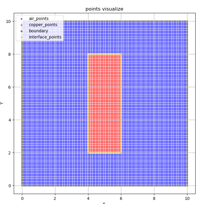
all_points = torch.cat([boundary, interface_points, copper_points,air_points], dim=0)def pointsplot():plt.figure(figsize=(8, 8))plt.scatter(air_points[:, 0].numpy(), air_points[:, 1].numpy(), s=10, c='blue', alpha=0.5,label='air_points')plt.scatter(copper_points[:, 0].numpy(), copper_points[:, 1].numpy(), s=10, c='red', alpha=0.5,label='copper_points')plt.scatter(boundary[:, 0].numpy(), boundary[:, 1].numpy(), s=10, c='black', alpha=0.5,label='boundary')plt.scatter(interface_points[:, 0].numpy(), interface_points[:, 1].numpy(), s=10, c='orange', alpha=0.5,label='interface_points')plt.xlabel('X ')plt.ylabel('Y')plt.title('points visualize')plt.legend()plt.grid(True)plt.show()# 打印各部分点数和总点数
print(f"边界点数: {boundary.shape[0]}")
print(f"界面点数: {interface_points.shape[0]}")
print(f"内部点数: {internal_points.shape[0]}")
print(f"总点数: {all_points.shape[0]}")
pointsplot()class layer(nn.Module):def __init__(self, n_in, n_out, activation):super().__init__()self.layer = nn.Linear(n_in, n_out)self.activation = activationdef forward(self, x):x = self.layer(x)if self.activation:x = self.activation(x)return xdef weights_init(m):if isinstance(m, nn.Linear):torch.nn.init.xavier_uniform_(m.weight.data)torch.nn.init.zeros_(m.bias.data)
class DNN(nn.Module):# dim_in 和 dim_out:分别为网络的输入和输出维度,n_layer 和 n_node:n_layer 表示隐藏层的数量, activation为激活函数,ub 和 lb:分别是区域的上界和下界,用于输入的归一化处理。def __init__(self, dim_in, dim_out, n_layer, n_node, activation = nn.Tanh()):super().__init__()self.net = nn.ModuleList()self.net.append(layer(dim_in, n_node, activation)) #第一个输入层for _ in range(n_layer):self.net.append(layer(n_node, n_node, activation))self.net.append(layer(n_node, dim_out, activation=None)) #最后一个输出层self.net.apply(weights_init) # weights_init 函数对网络的权重和偏置进行初始化(例如 Xavier 初始化),从而提供较好的初始收敛性。def forward(self, x):out = xfor layer in self.net:out = layer(out)return outclass PINN:def __init__(self) -> None:# 定义每个介质的网络self.nets = [DNN(dim_in=2, dim_out=1, n_layer=6, n_node=80).to(device),DNN(dim_in=2, dim_out=1, n_layer=6, n_node=80).to(device),# DNN(dim_in=2, dim_out=1, n_layer=6, n_node=50).to(device)]self.lbfgs = torch.optim.LBFGS(params=[p for net in self.nets for p in net.parameters()],lr=0.1,max_iter=20000,max_eval=20000,tolerance_grad=1e-5,tolerance_change= 1 * np.finfo(float).eps,history_size=50,line_search_fn="strong_wolfe",)#分别定义了 LBFGS 和 Adam 两种优化器。LBFGS 是一种基于二阶信息的优化算法,适用于物理信息神经网络的优化;Adam 是一种常用的一阶优化方法,用于更新网络权重。# self.adam = [# torch.optim.Adam(net.parameters(), lr=1e-4) for net in self.nets# ]self.adam = torch.optim.Adam(params=[p for net in self.nets for p in net.parameters()], lr=1e-5)self.losses = {"bc": [], "pde": [], "interface": [], "loss": []}self.iter = 0def predict(self, xy):output = torch.zeros(xy.shape[0], 1) # Ensure output has the right shapemask = pg.generate_mask(xy,4,2,6,8)output[mask] = self.nets[0](xy[mask])output[~mask] = self.nets[1](xy[~mask])return outputdef bc_loss(self):boundary.requires_grad = TrueA = self.predict(boundary)# 边界条件处理mse_bc = torch.mean(A**2)#边界损失l_bc = mse_bcreturn l_bcdef interface_bc_loss(self):"""计算公共边界条件损失函数"""interface_vertical.requires_grad = Trueinterface_horizontal.requires_grad = TrueA_interface_1_vertical = self.nets[0](interface_vertical)A_interface_2_vertical = self.nets[1](interface_vertical)A_interface_1_horizontal = self.nets[0](interface_horizontal)A_interface_2_horizontal = self.nets[1](interface_horizontal)# 第一边界条件l_1 = torch.mean(torch.square(A_interface_1_vertical - A_interface_2_vertical)) + torch.mean(torch.square(A_interface_1_horizontal - A_interface_2_horizontal))# 第二边界条件grad_1_vertical = grad(A_interface_1_vertical.sum(), interface_vertical, create_graph=True)[0][:, 0:1]grad_2_vertical = grad(A_interface_2_vertical.sum(), interface_vertical, create_graph=True)[0][:, 0:1]grad_1_horizontal = grad(A_interface_1_horizontal.sum(), interface_horizontal, create_graph=True)[0][:, 1:2]grad_2_horizontal = grad(A_interface_2_horizontal.sum(), interface_horizontal, create_graph=True)[0][:, 1:2]grad_1 = torch.cat([grad_1_vertical, grad_1_horizontal])grad_2 = torch.cat([grad_2_vertical, grad_2_horizontal])l_2 = torch.mean(torch.square(mu_copper*grad_1-mu_air*grad_2))return l_1+l_2def pde_loss(self, xy):xy = xy.clone().detach().requires_grad_(True)mask = pg.generate_mask(xy, 4, 2, 6, 8)# 铜导体区域xy_copper = xy[mask]A_copper = self.nets[0](xy_copper)grad_A_copper = grad(A_copper.sum(), xy_copper, create_graph=True)[0]dA_dx_copper = grad_A_copper[:, 0:1]dA_dy_copper = grad_A_copper[:, 1:2]d2A_dx2_copper = grad(dA_dx_copper.sum(), xy_copper, create_graph=True)[0][:, 0:1]d2A_dy2_copper = grad(dA_dy_copper.sum(), xy_copper, create_graph=True)[0][:, 1:2]nu_copper = 1 / (mu_copper)pde_copper = d2A_dx2_copper + d2A_dy2_copper + 1loss_copper = torch.mean((nu_copper * pde_copper) ** 2)# 空气区域xy_air = xy[~mask]A_air = self.nets[1](xy_air)grad_A_air = grad(A_air.sum(), xy_air, create_graph=True)[0]dA_dx_air = grad_A_air[:, 0:1]dA_dy_air = grad_A_air[:, 1:2]d2A_dx2_air = grad(dA_dx_air.sum(), xy_air, create_graph=True)[0][:, 0:1]d2A_dy2_air = grad(dA_dy_air.sum(), xy_air, create_graph=True)[0][:, 1:2]nu_air = 1 / (mu_air)pde_air = d2A_dx2_air + d2A_dy2_airloss_air = torch.mean((nu_air * pde_air) ** 2)return loss_copper + loss_airdef closure(self):self.lbfgs.zero_grad()self.adam.zero_grad()mse_bc = self.bc_loss()mse_pde = self.pde_loss(internal_points)mse_interface = self.interface_bc_loss()loss = mse_pde +mse_bc+mse_interfaceloss.backward()self.losses["bc"].append(mse_bc.detach().cpu().item())self.losses["pde"].append(mse_pde.detach().cpu().item())self.losses["interface"].append(mse_interface.detach().cpu().item())self.losses["loss"].append(loss.cpu().item())self.iter += 1print(f"\r It: {self.iter} Loss: {loss.item():.5e} BC: {mse_bc.item():.3e} PDE: {mse_pde.item():.3e} Interface: {mse_interface.item():.3e}",end="",)if self.iter % 100 == 0:print("")return lossdef save_model(self, path):"""保存模型和训练状态:param path: 保存文件路径"""save_dict = {"nets": [net.state_dict() for net in self.nets], # 保存所有子网络的参数"optimizers": [self.adam.state_dict(), self.lbfgs.state_dict()], # 保存优化器状态"losses": self.losses, # 保存损失记录"iteration": self.iter, # 保存当前迭代次数}torch.save(save_dict, path)print(f"模型已保存到 {path}")def load_model(self, path):"""加载模型和训练状态:param path: 加载文件路径"""checkpoint = torch.load(path, map_location=device)# 加载每个网络的参数for net, state_dict in zip(self.nets, checkpoint["nets"]):net.load_state_dict(state_dict)# 加载每个优化器的状态for opt, state_dict in zip([self.adam, self.lbfgs], checkpoint["optimizers"]):opt.load_state_dict(state_dict)# 加载其他训练状态self.losses = checkpoint["losses"]self.iter = checkpoint["iteration"]print(f"模型已从 {path} 加载")def plotLoss(losses_dict, path, info=["BC", "PDE","Interface","Loss"]):fig, axes = plt.subplots(1, 4, sharex=True, sharey=True, figsize=(12, 6))axes[0].set_yscale("log")for i, j in zip(range(4), info):axes[i].plot(losses_dict[j.lower()])axes[i].set_title(j)plt.show()fig.savefig(path)if __name__ == "__main__":pinn = PINN()start_time = time.time()for i in range(10000):pinn.closure()pinn.adam.step()pinn.lbfgs.step(pinn.closure)print("--- %s seconds ---" % (time.time() - start_time))print(f'-- {(time.time() - start_time)/60} mins --')now = datetime.datetime.now()# 格式化时间为字符串,例如:2024-11-28_15-30-00time_str = now.strftime("%m%d-%H%M")pinn.save_model( f"Param{time_str}.pt")plotLoss(pinn.losses, f"LossCurve{time_str}.png", )
预测代码
import numpy as np
import matplotlib.pyplot as plt
import torch
from main import PINN, mu0
from scipy.interpolate import griddatadevice = torch.device("cuda") if torch.cuda.is_available() else torch.device("cpu")pinn = PINN()
# 定义网格的分辨率
grid_size_x = 200
grid_size_y = 200
x_min = 0
x_max = 10
y_min =0
y_max = 10# 生成x和y坐标的等距网格点
x = np.linspace(x_min, x_max, grid_size_x)
y = np.linspace(y_min, y_max, grid_size_y)
X, Y = np.meshgrid(x, y)# 将网格点转化为输入格式(grid_size * grid_size, 2)
xy_grid = np.hstack((X.reshape(-1, 1), Y.reshape(-1, 1)))
xy_grid = torch.tensor(xy_grid, dtype=torch.float32).to(device)
time_str = '0531-1718'
pinn.load_model(f"Param{time_str}.pt")# 预测温度
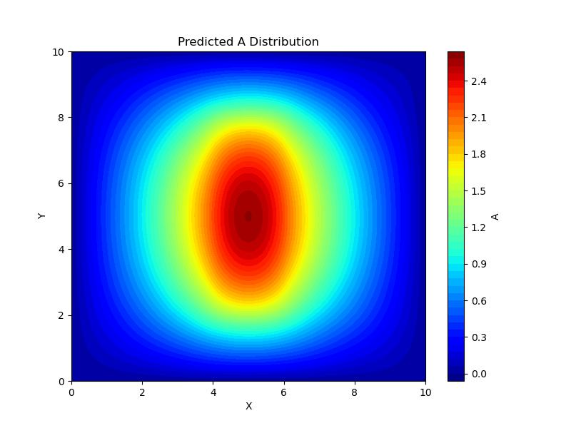
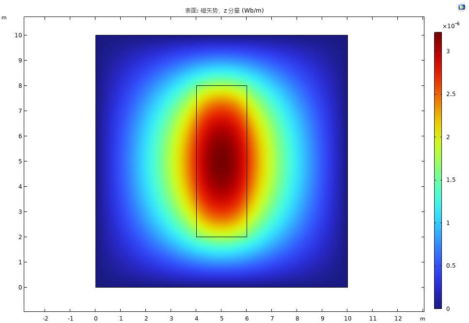
with torch.no_grad():A_pred = pinn.predict(xy_grid)*mu0# 将预测的温度值转化为numpy格式,并恢复为网格形状
A_pred = A_pred.detach().cpu().numpy().reshape(Y.shape)plt.figure(figsize=(8, 6))
plt.contourf(x,y,A_pred,levels=50, cmap='jet')
plt.colorbar(label='A')
plt.xlabel('X')
plt.ylabel('Y')
plt.title('Predicted A Distribution')
plt.savefig(f"Sol{time_str}.jpg")
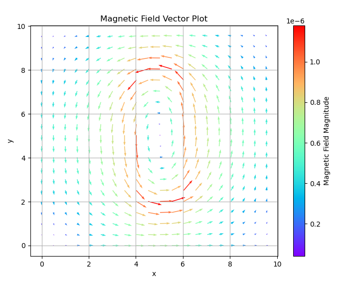
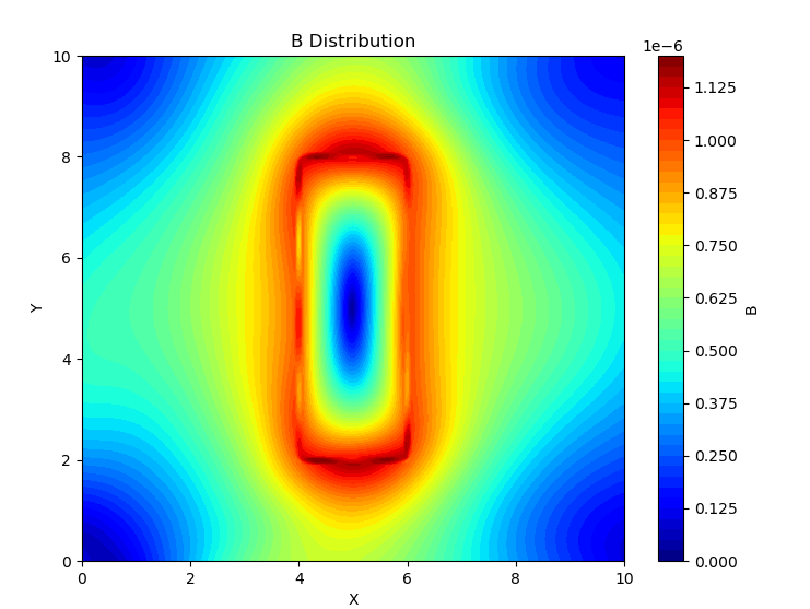
plt.show()# 计算磁场分量 Bx 和 By
Ay, Ax = np.gradient(A_pred, y, x)
Bx = Ay
By = -Ax
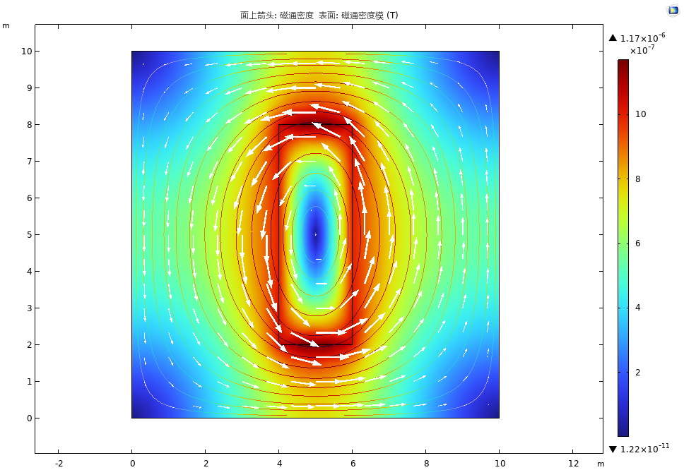
B = np.sqrt(Bx**2+By**2)skip = 10 # 每隔 skip 个点绘制一个箭头# 绘制磁场矢量图
plt.figure(figsize=(8, 6))
# 使用 B_magnitude 作为颜色的依据
quiver = plt.quiver(X[::skip, ::skip], Y[::skip, ::skip], Bx[::skip, ::skip], By[::skip, ::skip],B[::skip, ::skip], cmap='rainbow')
#设置图的背景色
# plt.gca().set_facecolor('black')
plt.colorbar(quiver, label='Magnetic Field Magnitude')
plt.title('Magnetic Field Vector Plot')
plt.xlabel('x')
plt.ylabel('y')
plt.grid()
plt.show()
如果代码运行有问题或对内容有疑问,都可以后台私信哦!
期待下一期PINNs案例代码分享吧!
基于物理信息的神经网络是一种解决偏微分方程计算问题的全新方法…
有关PINN基础详见:PINNs案例——中心热源温度场预测问题的torch代码
今日分享代码案例:二维带电流源磁场计算
该案例参考学习论文:
[1]张宇娇,孙宏达,赵志涛,徐斌,黄雄峰.基于物理信息神经网络的电磁场计算方法[J/OL].电工技术学报.
结果前瞻
问题场景
- **求解域:**案例选取边长为 10 的正方形区域作为研究对象,即定义域为
$ \Omega = [0, 10] \times [0, 10] 。以正方形左下角为原点,正方形区域内包含一个带电流密度为 1 的导体,导体区域为 。以正方形左下角为原点,正方形区域内包含一个带电流密度为1的导体,导体区域为 。以正方形左下角为原点,正方形区域内包含一个带电流密度为1的导体,导体区域为 \Omega = [4, 2] \times [6, 8] $。 - **参数设定:**导体处 J = 1 J = 1 J=1,导体材料为铜(copper),其余区域为空气(air),磁导率 γ \gamma γ 均为1
- **边界条件:**方形四周边界的矢量磁位为0(理想导体边界)
- **求解量:**区域内二维稳态磁场分布(矢量)
PINNs理论求解
在本案例中,我们引入矢量磁位 $ \mathbf{A} $ 来辅助磁场的计算。矢量磁位A设定为:
B = ∇ × A \mathbf{B} = \nabla \times \mathbf{A} B=∇×A
其中, B \mathbf{B} B 表示磁场强度,该关系表明磁场是矢量磁位的旋度。
在该正方形区域内,矢量磁位 $ A_z(x, y) $ 满足麦克斯韦方程,引入矢量磁位A后在二维稳态下,其数学表达式为:
( ∂ 2 A z ∂ x 2 + ∂ 2 A z ∂ y 2 ) = − μ J z \left( \frac{\partial^2 A_z}{\partial x^2} + \frac{\partial^2 A_z}{\partial y^2} \right) =-\mu J_z (∂x2∂2Az+∂y2∂2Az)=−μJz
其中:
- $ \mu $ 为材料的磁导率,表示材料对磁场的响应能力;
- $ J_z $ 为电流密度在 $ z $ 方向的分量,表示单位面积内电流的大小;
- $ A_z(x, y) $ 为矢量磁位在 $ z $ 方向的分量,通常用于描述二维平面内的磁场分布。
这种方程形式常见于静电学或静磁学中的泊松方程,用于描述在存在源(如电荷或电流)的情况下,势函数(如矢量磁位)的空间分布。矢量磁位的引入使得磁场的计算更为简便,尤其是在处理对称性问题或边界条件时。
本次案例中,由于存在铜导体区域(有源)和空气域(无源),故采用PINNs案例——多介质分区热传导中相同的分区思想。此处不过多介绍
损失函数可以表示为:
- **PDE 残差项:**控制方程如下:
Loss PDE = 1 N c ∑ i = 1 N c ∣ f ( x c i , y c i ) ∣ 2 \text{Loss}_{\text{PDE}} = \frac{1}{N_c} \sum_{i=1}^{N_c} \left| f\left( x_c^i, y_c^i \right) \right|^2 LossPDE=Nc1i=1∑Nc f(xci,yci) 2
f ( x c i , y c i ) = ( ∂ 2 A z ∂ x 2 + ∂ 2 A z ∂ y 2 ) + μ J z f\left( x_c^i, y_c^i \right) = \left( \frac{\partial^2 A_z}{\partial x^2} + \frac{\partial^2 A_z}{\partial y^2} \right) +\mu J_z f(xci,yci)=(∂x2∂2Az+∂y2∂2Az)+μJz
注意: 由于PDE损失中需加入 μ 0 \mu_{0} μ0,而 μ 0 = 4 π ∗ 10 − 7 \mu_{0} = 4\pi * 10^{-7} μ0=4π∗10−7 数量级过小,会对神经网络的训练带来较大困难。故需对PDE方程进行简单的无量纲化操作,令 A ′ = A / μ 0 A' = A/\mu_0 A′=A/μ0, 于是可以得到 f ( x c i , y c i ) = ( ∂ 2 A z ′ ∂ x 2 + ∂ 2 A z ′ ∂ y 2 ) + μ r J z f\left( x_c^i, y_c^i \right) = \left( \frac{\partial^2 A_z'}{\partial x^2} + \frac{\partial^2 A_z'}{\partial y^2} \right) +\mu_r J_z f(xci,yci)=(∂x2∂2Az′+∂y2∂2Az′)+μrJz.预测后再将A乘 μ 0 \mu_0 μ0以还原A
- 边界条件项:在多介质问题中,边界条件除矢量磁位A=0的方形边界条件,还要添加不同介质交界面的连续性边界条件。
-
固定温度边界:
Loss BC = 1 N b ∑ i = 1 N b ∣ A ( x b i , y b i ) ∣ 2 \text{Loss}_{\text{BC}} = \frac{1}{N_b} \sum_{i=1}^{N_b} \left|A\left( x_b^i, y_b^i \right) \right|^2 LossBC=Nb1i=1∑Nb A(xbi,ybi) 2 -
介质交界面:
此案例中以A的第一类和第二类边界条件作为介质交界面的连续性条件
第一类边界条件:
Loss I1 = 1 N I ∑ j = 1 N I ∣ A p ( x I j ) − A p + 1 ( x I j ) ∣ 2 \text{Loss}_{\text{I1}} = \frac{1}{N_{I}}\sum_{j=1}^{N_{I}}\left| A_{p}\left(x_{I}^{j}\right)-A_{p+1}\left(x_{I}^{j}\right)\right|^{2} LossI1=NI1j=1∑NI Ap(xIj)−Ap+1(xIj) 2
第二类边界条件(不同介质在边界面上矢量磁位法向导数与磁导率的乘积连续):
Loss I2 = 1 N I ∑ j = 1 N I ∣ γ p ∂ A p ( x I j ) ∂ n − γ p + 1 ∂ A p + 1 ( x I j ) ∂ n ∣ 2 \text{Loss}_{\text{I2}} = \frac{1}{N_{I}}\sum_{j=1}^{N_{I}}\left|\gamma_{p}\frac{\partial A_{p}\left(x_{I}^{j}\right)}{\partial n}-\gamma_{p+1}\frac{\partial A_{p+1}\left(x_{I}^{j}\right)}{\partial n}\right|^{2} LossI2=NI1j=1∑NI γp∂n∂Ap(xIj)−γp+1∂n∂Ap+1(xIj) 2
其中:
- $ N_I $ 表示介质边界点的点数
- $ A_p $ 表示第P个介质的矢量磁位
- $ \gamma_ {p} $ 表示第P个介质的热导率
训练
采用10000次adam优化与lbfgs优化器进行优化。各项损失收敛过程如下,收敛效果良好:
复现结果
comsol仿真结果
可见结果吻合良好
pytorch代码
为避免繁杂的点生成,作者编写了一组点生成函数,使用时单独建立points_generator.py,并在训练代码中引入。
points_generator.py
import numpy as np
from pyDOE import lhsdef generate_boundary_points(x_min, y_min, x_max, y_max, n):# 计算每条边上的点数num_points_x = int((x_max - x_min) * n) + 1num_points_y = int((y_max - y_min) * n) + 1# 生成每条边上的点bottom_edge = np.array([np.linspace(x_min, x_max, num_points_x), np.full(num_points_x, y_min)]).Ttop_edge = np.array([np.linspace(x_min, x_max, num_points_x), np.full(num_points_x, y_max)]).Tleft_edge = np.array([np.full(num_points_y, x_min), np.linspace(y_min, y_max, num_points_y)]).Tright_edge = np.array([np.full(num_points_y, x_max), np.linspace(y_min, y_max, num_points_y)]).T# 合并所有边上的点,去掉重复的角点boundary_points = np.concatenate([bottom_edge, top_edge[1:], left_edge[1:-1], right_edge[1:-1]])boundary_vertical = np.concatenate([left_edge[1:-1], right_edge[1:-1]])boundary_horizontal = np.concatenate([bottom_edge, top_edge[1:]])return boundary_points,boundary_vertical,boundary_horizontaldef generate_internal_points(x_min, y_min, x_max, y_max, n):# 计算内部点的网格x = np.linspace(x_min, x_max, int((x_max - x_min) * n) + 1)y = np.linspace(y_min, y_max, int((y_max - y_min) * n) + 1)x_grid, y_grid = np.meshgrid(x, y)# 去掉边界点x_grid = x_grid[1:-1, 1:-1]y_grid = y_grid[1:-1, 1:-1]# 将网格点转换为一维数组internal_points = np.array([x_grid.flatten(), y_grid.flatten()]).Treturn internal_pointsdef generate_mask(points, x_min, y_min, x_max, y_max):# 检查每个点是否在矩形区域内mask = (points[:, 0] >= x_min) & (points[:, 0] <= x_max) & (points[:, 1] >= y_min) & (points[:, 1] <= y_max)return maskdef lhs_internal_points(x_min, y_min, x_max, y_max, n):  '''使用超拉丁立方采样矩形区域内的点'''ub = np.array([x_max, y_max])lb = np.array([x_min, y_min])internal_points = lb + (ub - lb) * lhs(2, n)return internal_points
训练代码与预测代码请关注: