理解微积分 | 概念 / 定义 / 性质 / 关系

注：机翻，未全校。

以前的微积分基本概念笔记，出处未记录。

---

Calculus

微积分

The term Calculus is short for Calculus of the Infinitesimal. That means analyzing really tiny things in math that help us understand the bigger picture better.

微积分是“无穷小的微积分”的简称。这意味着通过分析数学中的非常微小的事物，帮助我们更好地理解整体的情况。

Differential Calculus

微分学

Differential Calculus deals with the concept of taking a derivative, also called differentiation. This means taking really small parts of a line to find the slope of a curve at every point.

微分学涉及导数的概念，也称为微分。这意味着将一条线分成非常小的部分，以求出曲线上每一点的斜率。

Integral Calculus

积分学

Integral Calculus deals with taking the Integral of a curve, also called integrating. This means splitting a curve into really small parts so that you can find the total area of the space under the whole curve.

积分学涉及对曲线进行积分，也称为积分运算。这意味着将曲线分成非常小的部分，以便求出整个曲线下的总面积。

These two concepts are tied together by the Fundamental theorem of calculus which essentially shows that these two seemingly separate operations are actually very closely tied together and are kind of inverses of each other.

这两个概念通过微积分基本定理联系在一起，该定理本质上表明，这两个看似独立的操作实际上密切相关，且互为逆运算。

---

Integration vs Differentiation

积分与微分

Integration and Differentiation are two fundamental concepts in calculus, which studies the change. Calculus has a wide variety of applications in many fields such as science, economy or finance, engineering and etc.
积分与微分是微积分中的两个基本概念，微积分研究的是变化。微积分在科学、经济或金融、工程等诸多领域有着广泛的应用。

Differentiation

微分

Differentiation is the algebraic procedure of calculating the derivatives. Derivative of a function is the slope or the gradient of the curve (graph) at any given point. Gradient of a curve at any given point is the gradient of the tangent drawn to that curve at the given point. For non - linear curves, the gradient of the curve can vary at different points along the axis. Therefore, it is difficult to calculate the gradient or the slope at any point. Differentiation process is useful in calculating the gradient of the curve at any point.
微分是计算导数的代数程序。函数的导数是曲线（图像）在任意给定点的斜率或梯度。曲线在任意给定点的梯度是该点处曲线的切线的梯度。对于非线性曲线，曲线的梯度可以在轴上的不同点变化。因此，计算任意点的梯度或斜率是困难的。微分过程有助于计算曲线在任意点的梯度。

Another definition for derivative is, “the change of a property with respect to a unit change of another property.”
导数的另一个定义是：“一个属性相对于另一个属性的单位变化的变化。”

Let $f(x)$ be a function of an independent variable $x$. If a small change $(\Delta x)$ is caused in the independent variable $x$, a corresponding change $\Delta f(x)$ is caused in the function $f(x)$; then the ratio $\frac{\Delta f(x)}{\Delta x}$ is a measure of rate of change of $f(x)$, with respect to $x$. The limit value of this ratio, as $\Delta x$ tends to zero, ${\lim }_{\Delta x\to 0}\frac{f(x)}{\Delta x}$ is called the first derivative of the function $f(x)$, with respect to $x$; in other words, the instantaneous change of $f(x)$ at a given point $x$.
设 $f(x)$ 是自变量 $x$ 的函数。如果自变量 $x$ 发生微小变化 $(\Delta x)$，函数 $f(x)$ 就会相应地发生变化 $\Delta f(x)$；那么比值 $\frac{\Delta f(x)}{\Delta x}$ 就是 $f(x)$ 相对于 $x$ 的变化率。当 $\Delta x$ 趋近于零时，这个比值的极限 ${\lim }_{\Delta x\to 0}\frac{f(x)}{\Delta x}$ 被称为函数 $f(x)$ 相对于 $x$ 的一阶导数；换句话说，它就是 $f(x)$ 在给定点 $x$ 处的瞬时变化。

Integration

积分

Integration is the process of calculating either definite integral or indefinite integral. For a real function $f(x)$ and a closed interval $[a,b]$ on the real line, the definite integral, ${\int }_a^{b}f(x)dx$, is defined as the area between the graph of the function, the horizontal axis and the two vertical lines at the end points of an interval. When a specific interval is not given, it is known as indefinite integral. A definite integral can be calculated using anti - derivatives.
积分是计算定积分或不定积分的过程。对于实函数 $f(x)$ 和实数轴上的闭区间 $[a,b]$，定积分 ${\int }_a^{b}f(x)dx$ 被定义为函数图像、水平轴以及区间端点处的两条垂直线之间的面积。如果没有给出具体的区间，则称为不定积分。定积分可以通过反导数来计算。

What is the difference between Integration and Differentiation?

积分与微分有何不同？

The difference between integration and differentiation is somewhat like the difference between “squaring” and “taking the square root.” If we square a positive number and then take the square root of the result, the positive square root value will be the number that you squared. Similarly, if you apply the integration to the result that you obtained by differentiating a continuous function $f(x)$, it will lead back to the original function and vice versa.
积分与微分的差异有点像“平方”与“开平方”的差异。如果我们对一个正数进行平方，然后对结果开平方，那么正平方根的值就是你平方的那个数。同样，如果你对一个连续函数 $f(x)$ 的导数结果进行积分，它会回到原来的函数，反之亦然。

For example, let $F(x)$ be the integral of function $f(x)=x$, therefore, $F(x)=\int f(x)dx=\frac{x^2}{2}+c$, where $c$ is an arbitrary constant. When differentiating $F(x)$ with respect to $x$ we get, $F^{\prime }(x)=\frac{dF(x)}{dx}=\frac{2x}{2}+0=x$, therefore, the derivative of $F(x)$ is equal to $f(x)$.
例如，设 $F(x)$ 是函数 $f(x)=x$ 的积分，因此，$F(x)=\int f(x)dx=\frac{x^2}{2}+c$，其中 $c$ 是任意常数。当我们对 $F(x)$ 求导时，得到 $F^{\prime }(x)=\frac{dF(x)}{dx}=\frac{2x}{2}+0=x$，因此，$F(x)$ 的导数等于 $f(x)$。

Summary

总结

• Differentiation calculates the slope of a curve, while integration calculates the area under the curve.
  微分计算曲线的斜率，而积分计算曲线下的面积。
• Integration is the reverse process of differentiation and vice versa.
  积分是微分的逆过程，反之亦然。

---

Calculus Summary

微积分总结

Calculus has two main parts: differential calculus and integral calculus. Differential calculus studies the derivative and integral calculus studies (surprise!) the integral. The derivative and integral are linked in that they are both defined via the concept of the limit: they are inverse operations of each other (a fact sometimes known as the fundamental theorem of calculus); and they are both fundamental to much of modern science as we know it.

微积分主要有两部分：微分学和积分学。微分学研究导数，而积分学（你可能猜到了！）研究积分。导数和积分相互关联，它们都是通过极限的概念来定义的；它们彼此是逆运算（这一事实有时被称为微积分基本定理）；并且它们对于我们所知的许多现代科学来说都是基础。

Derivatives

导数

The limit of a function $f(x)$ as $x$ approaches $a$ is equal to $b$ if for every desired closeness to $b$, you can find a small interval around (but not including) $a$ that achieves that closeness when mapped by $f$. Limits give us a firm mathematical basis on which to examine both the infinite and the infinitesimal. They are also easy to handle algebraically:

如果对于每一个期望接近 $b$ 的程度，都能找到一个围绕（但不包含）$a$ 的小区间，当通过 $f$ 映射时能达到该接近程度，那么函数 $f(x)$ 在 $x$ 趋近于 $a$ 时的极限等于 $b$。极限为我们研究无穷大和无穷小提供了坚实的数学基础。它们在代数运算上也很容易处理：

$$li{m}_{x\to a}[f(x)+g(x)]=li{m}_{x\to a}f(x)+li{m}_{x\to a}g(x)$$

$$li{m}_{x\to a}[f(x)g(x)]=\left[li{m}_{x\to a}f(x)\right]\left[li{m}_{x\to a}g(x)\right]$$

$$li{m}_{x\to a}c=c,$$

where in the last equation, $c$ is a constant and in the first two equations, if both limits of $f$ and $g$ exist.

在最后一个等式中，$c$ 是一个常数，在前两个等式中，要求 $f$ 和 $g$ 的极限都存在。

One important fact to keep in mind is that

需要记住的一个重要事实是

$$li{m}_{x\to a}f(x)$$

doesn’t depend at all on $f(a)$ – in fact, $f(a)$ is frequently undefined. In the happy case where

${\lim }_{x\to a}f(x)$ 完全不依赖于 $f(a)$ ，实际上，$f(a)$ 常常是没有定义的。在理想情况下，当

$$li{m}_{x\to a}f(x)=f(a)$$

we say that $f$ is continuous at $a$. It is also sometimes useful to talk about one - sided (left or right) limits, where we only care about the values of $x$ that are less than or greater than $a$.

我们就说 $f$ 在 $a$ 点连续。有时讨论单侧（左或右）极限也很有用，在单侧极限中，我们只关心 $x$ 小于或大于 $a$ 的值。

The derivative of $f(x)$ at $x=a$ (or $f^{\prime }(a)$) is defined as

$f(x)$ 在 $x=a$ 处的导数（或 $f^{\prime }(a)$ ）定义为

$$f^{\prime }(a)=li{m}_{x\to a}\frac{f(x)-f(a)}{x-a}$$

wherever the limit exists. The derivative has many interpretations and applications, including velocity (where $f$ gives position as a function of time), instantaneous rate of change, or slope of a tangent line to the graph of $f$. Using the algebraic properties of limits, you can prove these extremely important algebraic properties of derivatives:

只要该极限存在。导数有许多解释和应用，包括速度（其中 $f$ 将位置表示为时间的函数）、瞬时变化率，或者 $f$ 的图像切线的斜率。利用极限的代数性质，可以证明这些极其重要的导数代数性质：

$${\left(f+g\right)}^{\prime }=f^{\prime }+g^{\prime }$$

$$(c{)}^{\prime }=0c\text{ a constant}（c为常数）$$

$$(cf{)}^{\prime }=c{f}^{\prime }c\text{ a constant}（c为常数）$$

$${\left(x^n\right)}^{\prime }=n{x}^{n-1}n\text{ a positive integer}（n为正整数）$$

$$(fg{)}^{\prime }=f^{\prime }g+f{g}^{\prime }$$

$${\left(\frac{f}{g}\right)}^{\prime }=\frac{\left(f^{\prime }g-f{g}^{\prime }\right)}{(g{)}^2}$$

$$(f(g(x)){)}^{\prime }=g^{\prime }(x)f^{\prime }(g)theChainRule.（链式法则）$$

These rules, for example, allow you to calculate the derivative of any rational (= ratio of two polynomials) function. The chain rule in particular has many applications. For one thing, if you have two inverse functions $f$ and $g$, that is if $f(g(x))=x$, then the chain rule implies that $f^{\prime }(g)=\frac{1}{g^{\prime }(x)}$。

例如，这些规则能让你计算任何有理函数（即两个多项式的比值）的导数。链式法则尤其有很多应用。一方面，如果你有两个反函数 $f$ 和 $g$，即 $f(g(x))=x$ ，那么根据链式法则可得 $f^{\prime }(g)=\frac{1}{g^{\prime }(x)}$。

Also, if you have an implicitly defined function between $x$ and $y$ like $x^2-2xy+y^2=1$, then you can perform implicit differentiation (basically, just taking the derivative of everything with respect to both $x$ and $y$ and tacking on $dx$ s and $dy$ s to indicate which) to get $2xdx-2xdy-2ydx+2ydy=0$. Then if you solve for $\frac{dy}{dx}$, this will be equal (by the chain rule) to $y^{\prime }$ and if you solve for $\frac{dx}{dy}$, this will be equal to $x^{\prime }$. Note that in this case, either derivative will be in terms of both $x$ and $y$.

另外，如果你有一个 $x$ 和 $y$ 之间的隐函数，如 $x^2-2xy+y^2=1$ ，那么你可以进行隐函数求导（基本上就是对所有项分别关于 $x$ 和 $y$ 求导，并加上 $dx$ 和 $dy$ 来表明是对哪个变量求导），得到 $2xdx-2xdy-2ydx+2ydy=0$。然后，如果你求解 $\frac{dy}{dx}$ ，根据链式法则，它将等于 $y^{\prime }$；如果你求解 $\frac{dx}{dy}$ ，它将等于 $x^{\prime }$。注意，在这种情况下，任何一个导数都将用 $x$ 和 $y$ 来表示。

You may be wondering about the derivatives of your favorite trigonometric functions. Well,

你可能想知道你喜欢的三角函数的导数。嗯，

$$(sin(x){)}^{\prime }=cos(x)\text{ and }(cos(x){)}^{\prime }=-sin(x).$$

These two facts, combined with the rules above, allow one to calculate easily the derivatives of the rest of the trigonometric functions and their inverses. The derivatives of the hyperbolic functions are similar, except that

这两个事实，结合上面的规则，能让人轻松计算出其余三角函数及其反函数的导数。双曲函数的导数与之类似，只是

$$(sinh(x){)}^{\prime }=cosh(x)\text{ and }(cosh(x){)}^{\prime }=sinh(x).$$

Many physical applications of derivatives reduce to finding solutions to differential equations: equations relating a function and its derivatives. For example, both sine and cosine satisfy the differential equation $f^{\prime \prime }(x)=-f(x)$, which models ideal pendulums, springs, and other examples of simple harmonic motion. The equation $f^{\prime }(x)=kf(x)$ comes up in modeling population growth and radioactive decay, and is solved by the function $f(x)=e^{kx}$, where

导数在许多物理应用中归结为求解微分方程：即关联一个函数及其导数的方程。例如，正弦函数和余弦函数都满足微分方程 $f^{\prime \prime }(x)=-f(x)$ ，该方程用于模拟理想摆、弹簧以及其他简谐运动的例子。方程 $f^{\prime }(x)=kf(x)$ 出现在人口增长和放射性衰变的建模中，其解为函数 $f(x)=e^{kx}$ ，其中

$$e=li{m}_{n\to \infty }{\left(1+\frac{1}{n}\right)}^n=\mathrm{2.7182...}$$

is called Euler’s constant and is defined to be the unique real number $e$ such that $(e^x{)}^{\prime }=e^x$. The inverse of the exponential function $e^x$ is the natural logarithm function $\log (x)$, which has many useful and interesting properties, including:

被称为欧拉常数，它被定义为唯一的实数 $e$ ，使得 $(e^x{)}^{\prime }=e^x$。指数函数 $e^x$ 的反函数是自然对数函数 $\log (x)$ ，它有许多有用且有趣的性质，包括：

$$-\log (ab)=\log a+\log b$$

[This way logarithms turn multiplications into into additions was why log tables (and their analog cousins, slide rules) were used to do long multiplications before computers came along.]

[对数将乘法转化为加法，这就是在计算机出现之前，对数表（以及类似的计算尺）被用于进行长乘法运算的原因。]

• $\log (a/b)=\log a-\log b$

• $e^{(\log x)}=x\text{ and }\log e^x=x$

• $\log x^a=a\log x$

• $a^x=e^{(x\log a)}$

• $(\log (x){)}^{\prime }=\frac{1}{x}$

• $\log 1=0$

Closely related to the natural logarithm is the logarithm to the base $b$, $({\log }_{b}x)$, which can be defined as $\log (x)/\log (b)$.

与自然对数密切相关的是以 $b$ 为底的对数 $({\log }_{b}x)$ ，它可以定义为 $\log (x)/\log (b)$。

Finally, derivatives can be used to help you graph functions. First, they give you the slope of the graph at a point, which is useful. Second, the points where the slope of the graph is horizontal ($f^{\prime }(x)=0$) are particularly important, because these are the only points at which a relative minimum or maximum can occur (in a differentiable function). These points where $f^{\prime }(x)=0$ are called critical points. To determine whether a critical point is a minimum or maximum, or more generally to determine the concavity of a function, second derivatives can be used; $f^{\prime \prime }(x)<0$ means a relative maximum/concave down, $f^{\prime \prime }(x)>0$ means a relative minimum /concave up. Finally, taking the limit as $x$ goes to positive or negative infinity gives information about the function’s asymptotic behavior. Towards that end, derivatives can help you out with some difficult limits: by L’Hôpital’s rule, if $\lim f(x)$ and $\lim g(x)$ are both zero, then $\lim \frac{f(x)}{\lim g(x)}=\lim \frac{f^{\prime }(x)}{\lim g^{\prime }(x)}$. The proof of L’Hôpital’s rule relies on the Mean Value Theorem: that for any function $f(x)$ differentiable between $a$ and $b$, there is some point $c$ between $a$ and $b$ such that the derivative of $f$ at $c$ is the same as the average slope between $a$ and $b$:

最后，导数可以帮助你绘制函数图像。首先，它能给出函数图像在某一点的斜率，这很有用。其次，函数图像斜率为水平的点（$f^{\prime }(x)=0$）尤为重要，因为在可导函数中，这些点是仅有的可能出现相对最小值或最大值的点。这些 $f^{\prime }(x)=0$ 的点被称为临界点。为了判断一个临界点是最小值点还是最大值点，或者更一般地判断函数的凹凸性，可以使用二阶导数；$f^{\prime \prime }(x)<0$ 表示相对最大值 / 下凹，$f^{\prime \prime }(x)>0$ 表示相对最小值 / 上凸。最后，求 $x$ 趋于正无穷或负无穷时的极限，可以得到函数的渐近行为信息。为此，导数可以帮助你求解一些困难的极限：根据洛必达法则，如果 $\lim f(x)$ 和 $\lim g(x)$ 都为零，那么 $\lim \frac{f(x)}{\lim g(x)}=\lim \frac{f^{\prime }(x)}{\lim g^{\prime }(x)}$。洛必达法则的证明依赖于洛必达法则依赖于中值定理：对于在 $a$ 和 $b$ 之间可导的任何函数 $f(x)$ ，在 $a$ 和 $b$ 之间存在某个点 $c$ ，使得 $f$ 在 $c$ 点的导数与 $a$ 和 $b$ 之间的平均斜率相同：

$$f^{\prime }(c)=\frac{f(b)-f(a)}{b-a}$$

Integrals

积分

The integral of $f(x)$ from $a$ to $b$ with respect to $x$ is noted as

$f(x)$ 从 $a$ 到 $b$ 关于 $x$ 的积分记为

$${\int }_a^{b}f(x)dx$$

and gives the area under the graph of $f$ and above the interval $[a,b]$. It can be defined formally as a Riemann sum: the limit of the areas of rectangular approximations to the area as the approximations get better and better.

它表示 $f$ 的图像在区间 $[a,b]$ 上方的面积。它可以正式定义为黎曼和：即矩形逼近面积的极限，随着逼近程度越来越好。

As stated before, integration and differentiation are inverse operations. To be precise, the fundamental theorem of calculus states that

如前所述，积分和微分是逆运算。确切地说，微积分基本定理指出

$${\int }_a^b{f}^{\prime }(x)dx=f(b)-f(a)\text{ and }{\left({\int }_a^{x}f(z)dz\right)}^{\prime }=f(x).$$

More generally, using an application of the Chain Rule,

更一般地，应用链式法则可得

$${\left({\int }_{g(x)}^{h(x)}f(z)dz\right)}^{\prime }=f(h(x))h^{\prime }(x)-f(g(x))g^{\prime }(x).$$

Knowing these facts, we now know a tremendous number of integrals: just flip the sides of any table of derivatives. Here are some further facts about integrals:

了解了这些事实后，我们现在知道了大量的积分：只需将任何导数表的两边互换即可。以下是关于积分的一些更多事实：

$${\int }_a^b[f(x)\pm g(x)]dx={\int }_a^{b}f(x)dx\pm {\int }_a^{b}g(x)dx$$

For $c$ a constant,

对于常数 $c$，

$${\int }_a^{b}cf(x)dx=c{\int }_a^{b}f(x)dx$$

$${\int }_a^{c}f(x)dx={\int }_a^{b}f(x)dx+{\int }_b^{c}f(x)dx$$

The integral of a positive, continuous function from $a$ to $b$ with $b>a$ is greater than zero.

当 $b>a$ 时，一个在区间 $[a,b]$ 上的正的连续函数的积分大于零。

The integral from $a$ to $b$ of $f(x)-g(x)$, with $f(x)>g(x)$ in the interval $[a,b]$ gives the area between $f(x)$ and $g(x)$∶

当在区间 $[a,b]$ 上 $f(x)>g(x)$ 时，$f(x)-g(x)$ 从 $a$ 到 $b$ 的积分表示 $f(x)$ 和 $g(x)$ 之间的面积：

If those properties aren’t enough to solve your integral, and if you can’t find it in any table, then here are some further tricks of the trade:

如果这些性质不足以求解你的积分，并且你在任何积分表中都找不到它，那么这里有一些更多的常用技巧：

Substitution (the “inverse” of the Chain Rule):

换元法（链式法则的 “逆运算”）：

$${\int }_a^b(f(u(x)){)}^{\prime }dx={\int }_a^{b}f(u)du$$

Integration by parts (the “inverse” of the Product Rule):

分部积分法（乘积法则的 “逆运算”）：

$${\int }_a^b{f}^{\prime }(x)g(x)=f(b)g(b)-f(a)g(a)-{\int }_a^{b}f(x)g^{\prime }(x)dx.$$

Partial fractions: Every rational function with a denominator which can be broken up into the sum of fractions of the form

部分分式法：每一个分母可以分解为以下形式的分式之和的有理函数

$$\frac{A}{Bx+C}\text{ or }\frac{Ax+B}{C{x}^2+Dx+E},$$

where $A$, $B$, $C$, $D$ and $E$ are constants (of course not the same constants in the two forms) may be (more) easily integrated.

其中 $A$、$B$、$C$、$D$ 和 $E$ 是常数（当然，两种形式中的常数不同），这样的函数可能更容易积分。

Numerical approximation. This may not give you give you an exact answer, but approximating the area under $f(x)$ with rectangles, trapezoids, or even more complicated shapes can give you a value near the integral when no other method will work. For a brief explanation of the use of an application available to MIT students, see Definite Integrals on Maple, part of Using Maple for ESG Subjects, used as part of the MIT subject 18.01A at ESG.

数值逼近法。这可能无法给你一个精确答案，但当其他方法都行不通时，用矩形、梯形甚至更复杂的形状来逼近 $f(x)$ 下方的面积，可以得到接近积分值的结果。关于麻省理工学院学生可用的一个应用程序的简要说明，可查看 “Maple 中的定积分”，它是 “ESG 学科使用 Maple” 的一部分，用于麻省理工学院 ESG 的 18.01A 课程。

Integrals are defined to find areas, but they can also be used to calculate other measure properties such as length or volume. For instance, the integral

积分被定义用于求面积，但它们也可以用于计算其他度量属性，如长度或体积。例如，积分

$${\int }_a^b\sqrt{1+{\left(f^{\prime }(x)\right)}^2}dx$$

gives the arclength of the graph of $f(x)$ between $x=a$ and $x=b$. The integral

给出了 $f(x)$ 的图像在 $x=a$ 和 $x=b$ 之间的弧长。积分

$${\int }_a^b\pi (f(x){)}^{2}dx$$

gives the volume contained by revolving the graph of $f(x)$ between $x=a$ and $x=b$ about the $x$-axis. The integral

给出了 $f(x)$ 的图像在 $x=a$ 和 $x=b$ 之间绕 $x$ 轴旋转所围成的体积。积分

$${\int }_a^{b}2\pi xf(x)dx$$

gives the volume contained by revolving the graph of $f(x)$ between $x=a$ and $x=b$ about the $y$-axis. Finally, the surface area of the surface formed by revolving the graph of $f(x)$ between $x=a$ and $x=b$ about the $x$-axis can be found by the integral

给出了 $f(x)$ 的图像在 $x=a$ 和 $x=b$ 之间绕 $y$ 轴旋转所围成的体积。最后，$f(x)$ 的图像在 $x=a$ 和 $x=b$ 之间绕 $x$ 轴旋转所形成的曲面的表面积可以通过积分

$${\int }_a^{b}2\pi f(x)\sqrt{1+{\left(f^{\prime }(x)\right)}^2}dx$$

Sometimes you will wish to take an integral over an unbounded interval such as from $1$ to infinity, or to take an integral of a function that is undefined at some points (such as $\frac{1}{\sqrt{x}}$). These are improper integrals, and can be found by taking the limit of an integral over an interval that either grows towards infinity or towards the points where the function is undefined.

有时你可能想要计算在无界区间上的积分，比如从 $1$ 到无穷大，或者计算在某些点无定义的函数（比如 $\frac{1}{\sqrt{x}}$ ）的积分。这些是反常积分，可以通过取积分区间趋向于无穷大或趋向于函数无定义点的极限来求解。

---

The Definition of Differentiation

微分的定义

The essence of calculus is the derivative. The derivative is the instantaneous rate of change of a function with respect to one of its variables. This is equivalent to finding the slope of the tangent line to the function at a point. Let’s use the view of derivatives as tangents to motivate a geometric definition of the derivative.

微积分的核心是导数。导数是函数相对于其某个变量的瞬时变化率。这等同于求函数在某一点处切线的斜率。让我们从导数是切线斜率这一观点出发，来引出导数的几何定义。

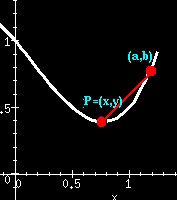
We want to find the slope of the tangent line to a graph at the point $P$. We can approximate the slope by drawing a line through the point $P$ and another point nearby, and then finding the slope of that line, called a secant line. The slope of a line is determined using the following formula (where $m$ represents slope):

我们想要找到函数图像在点 $P$ 处切线的斜率。我们可以通过过点 $P$ 和附近另一个点画一条线，然后求出这条线（称为割线）的斜率来近似切线斜率。直线的斜率由以下公式确定（其中 $m$ 表示斜率）：

$$m=\frac{rise}{run}=\frac{\Delta y}{\Delta x}.$$

Let $P=(x,y)$ and $Q:=(a,b)$. Let
设 $P=(x,y)$，$Q:=(a,b)$。令

$$a=x+\Delta x\text{ and }b=y+\Delta y=f(a)=f(x+\Delta x).$$

Then the slope of the line $\overline{PQ}$ is
那么直线 $\overline{PQ}$ 的斜率为

$$\frac{b-y}{a-x}=\frac{\Delta y}{\Delta x}=\frac{f(x+\Delta x)-f(x)}{\Delta x}.$$

Now, we chose an arbitrary interval to be $\Delta x$. How does the size of $\Delta x$ affect our estimate of the slope of the tangent line? The smaller $\Delta x$ is, the more accurate this approximation is. There is a wonderful animation of this by Douglas Arnold. Look at it here. You can see on the left of the animation how $\Delta x$ decreases, causing the secant line to approach the tangent, where it zooms in on the right. Another animation of this (also from Douglas Arnold) is here.

现在，我们任意选择了一个区间 $\Delta x$。$\Delta x$ 的大小是如何影响我们对切线斜率的估计的呢？$\Delta x$ 越小，这个近似就越精确。道格拉斯・阿诺德（Douglas Arnold）制作了一个很棒的动画展示这个过程。在这里查看 。在动画的左边，你可以看到 $\Delta x$ 是如何减小的，这使得割线逐渐接近切线，动画右边是放大后的效果。另一个相关动画（同样来自道格拉斯・阿诺德）在这里 。

What we want to do is decrease the size of $\Delta x$ as much as possible. We do this by taking the limit as $\Delta x$ approaches zero. In the limit, assuming the limit exists, we will find the exact slope of the tangent line to the curve at the given point. This value is the derivative;

我们想要尽可能地减小 $\Delta x$ 的大小。我们通过取 $\Delta x$ 趋近于 $0$ 时的极限来实现这一点。在这个极限过程中，如果极限存在，我们就能得到曲线在给定点处切线的精确斜率。这个值就是导数：

$$\frac{df}{dx}=\underset{\Delta x\to 0}{\lim }\frac{f(x+\Delta x)-f(x)}{\Delta x}.$$

There are a few different, but equivalent, versions of this definition. In more general considerations, $h$ is often used in place of $\Delta x$. Or $\Delta y$ is used in place of $f(x+\Delta x)-f(x)$. This leads to three commonly used ways of expressing the definition of the derivative:

这个定义有几种不同但等价的表述形式。在更普遍的讨论中，通常用 $h$ 来代替 $\Delta x$ 。或者用 $\Delta y$ 来代替 $f(x+\Delta x)-f(x)$。这就产生了三种常用的导数定义表达方式：

1. $\frac{df}{dx}={\lim }_{\Delta x\to 0}\frac{f(x+\Delta x)-f(x)}{\Delta x}$，which is the form we derived based on the geometric idea of the slope of the tangent line. Here, $\Delta x$ represents the small change in the independent variable $x$, and $f(x+\Delta x)-f(x)$ is the corresponding change in the function $y=f(x)$. As $\Delta x$ gets closer and closer to $0$, the ratio $\frac{f(x+\Delta x)-f(x)}{\Delta x}$ approaches the exact slope of the tangent line at the point $x$, which is the value of the derivative $\frac{df}{dx}$.

   $\frac{df}{dx}={\lim }_{\Delta x\to 0}\frac{f(x+\Delta x)-f(x)}{\Delta x}$，这是我们基于切线斜率的几何概念推导出来的形式。这里，$\Delta x$ 表示自变量 $x$ 的微小变化，$f(x+\Delta x)-f(x)$ 是函数 $y=f(x)$ 相应的变化量。当 $\Delta x$ 越来越接近 $0$ 时，比值 $\frac{f(x+\Delta x)-f(x)}{\Delta x}$ 趋近于点 $x$ 处切线的精确斜率，也就是导数 $\frac{df}{dx}$ 的值。

2. $\frac{df}{dx}={\lim }_{h\to 0}\frac{f(x+h)-f(x)}{h}$. This is just a notational variation of the first form. Using $h$ instead of $\Delta x$ is a matter of convention, and it is widely adopted in mathematical literature. For example, when proving derivative rules or calculating derivatives in more complex functions, this form can sometimes make the algebraic manipulations more straightforward.

   $\frac{df}{dx}={\lim }_{h\to 0}\frac{f(x+h)-f(x)}{h}$。这只是第一种形式在符号上的变化。用 $h$ 代替 $\Delta x$ 是一种惯例，在数学文献中被广泛采用。例如，在证明求导法则或计算更复杂函数的导数时，这种形式有时能使代数运算更简便。

3. $\frac{dy}{dx}={\lim }_{\Delta x\to 0}\frac{\Delta y}{\Delta x}$. Since $\Delta y=f(x+\Delta x)-f(x)$, this form emphasizes the relationship between the change in the dependent variable $y$ ($\Delta y$) and the change in the independent variable $x$ ($\Delta x$). It gives an intuitive sense of how the function $y=f(x)$ changes with respect to $x$ at a very small scale. When $\Delta x$ is extremely small, $\frac{\Delta y}{\Delta x}$ approximates the rate of change of $y$ with respect to $x$, and in the limit as $\Delta x\to 0$, it becomes the derivative $\frac{dy}{dx}$.

   $\frac{dy}{dx}={\lim }_{\Delta x\to 0}\frac{\Delta y}{\Delta x}$。因为 $\Delta y=f(x+\Delta x)-f(x)$，这种形式强调了因变量 $y$ 的变化量（$\Delta y$）和自变量 $x$ 的变化量（$\Delta x$）之间的关系。它直观地体现了函数 $y=f(x)$ 在极小尺度下随 $x$ 的变化情况。当 $\Delta x$ 极其小时，$\frac{\Delta y}{\Delta x}$ 近似表示 $y$ 关于 $x$ 的变化率，当 $\Delta x$ 趋于 $0$ 时，它就成为了导数 $\frac{dy}{dx}$ 。

Derivatives of Inverse Functions

反函数的导数

Suggested Prerequesites:

建议先修知识：
 
Inverse Functions, Implicit Differentiation, Chain Rule

反函数、隐函数求导、链式法则

Sometimes it may be more convenient or even necessary to find the derivative
有时，求导数可能会更方便，甚至是必要的。

$$\frac{d}{dx}g(x)$$

based on the knowledge or condition that
基于这样的知识或条件

$$g(x)=f^{-1}(x)$$

for some function $f(t)$, or, in other words, that $g(x)$ is the inverse of $f(t)=x$.
对于某个函数 $f(t)$ ，换句话说，$g(x)$ 是 $f(t)=x$ 的反函数

Then, recognizing that $t$ and $g(x)$ represent the same quantity, and remembering the Chain Rule,
然后，考虑到 $t$ 和 $g(x)$ 表示相同的量，并记住链式法则

$t=f^{-1}(x)$

$f(t)=x$

$\frac{d}{dx}f(t)=\frac{d}{dx}x$

$\frac{df}{dt}\frac{dt}{dx}=1$

$\frac{dt}{dx}=\frac{d}{dx}{f}^{-1}(x)=\frac{1}{\frac{df}{dt}}$

Using Leibniz’s fraction notation for derivatives, this result becomes somewhat obvious;

用莱布尼茨的导数分式记号表示，这个结果就变得很直观：

$$\frac{dy}{dx}=\frac{1}{\left(\frac{dx}{dy}\right)}$$

As with the chain rule, the Leibnitz notation can often provide insight that can be confirmed using the definition of the derivative or previously proven results.

和链式法则一样，莱布尼茨记号常常能让我们直观理解，并且可以用导数的定义或之前证明过的结论来验证。

What the above does not indicate, and which will be shown via the following examples, is that when the derivative of an inverse function is desired as a function of (in the above and following cases) the independent variable $x$, the derivative $\frac{dx}{dy}$ must be solved for $x$.

上述内容没有指出的是（下面的例子会说明），当我们想把反函数的导数表示成（在上述及下面的例子中）自变量 $x$ 的函数时，必须把 $\frac{dx}{dy}$ 用 $x$ 表示出来。

Some examples:

一些例子：

The following examples will be confined to those functions that can be differentiated by use of the Power Rule and the Chain Rule in combination.

下面的例子仅限于那些可以结合幂函数求导法则和链式法则进行求导的函数。

First, consider
首先，考虑

$$y=g(x)=\sqrt{x}=f^{-1}(x),f(y)=y^2$$

We know from the Power Rule, with $n=2$, that
根据幂函数求导法则（$n=2$ 时），我们知道

$$\frac{d}{dx}g(x)=\frac{1}{2\sqrt{x}}$$

Equivalently,
同样地，

$$\begin{array}{rl}\frac{dy}{dx}& =\frac{1}{\frac{df}{dy}}\\ & =\frac{1}{2y}\\ & =\frac{1}{2\sqrt{x}}\end{array}$$

as before.
如上

The above may be generalized; for nonzero $n$,
上述情况可以推广；对于非零的 $n$ ，

$$y=g(x)=x^n=f^{-1}(x),f(y)=y^{\frac{1}{n}}$$

Then,
那么，

$$\begin{array}{rl}\frac{dy}{dx}& =\frac{1}{\frac{df}{dy}}\\ & =\frac{1}{(\frac{1}{n})y^{(\frac{1}{n})-1}}\\ & =\frac{n}{x^{n((\frac{1}{n})-1)}}\\ & =n{x}^{n-1}\end{array}$$

in agreement with the Power Rule.
这与幂函数求导法则一致。