当前位置：首页 > ds >正文

HDRnet——双边滤波和仿射变换的摇身一变

ds 2025/5/8 21:20:44

主页：Deep Bilateral Learning

paper：https://groups.csail.mit.edu/graphics/hdrnet/data/hdrnet.pdf

coeffs

这部分的处理对象是低分辨率图，利用CNN进行特征提取（局部和全局），最后fuse得到grid，这里面包含了变换的系数。

splat

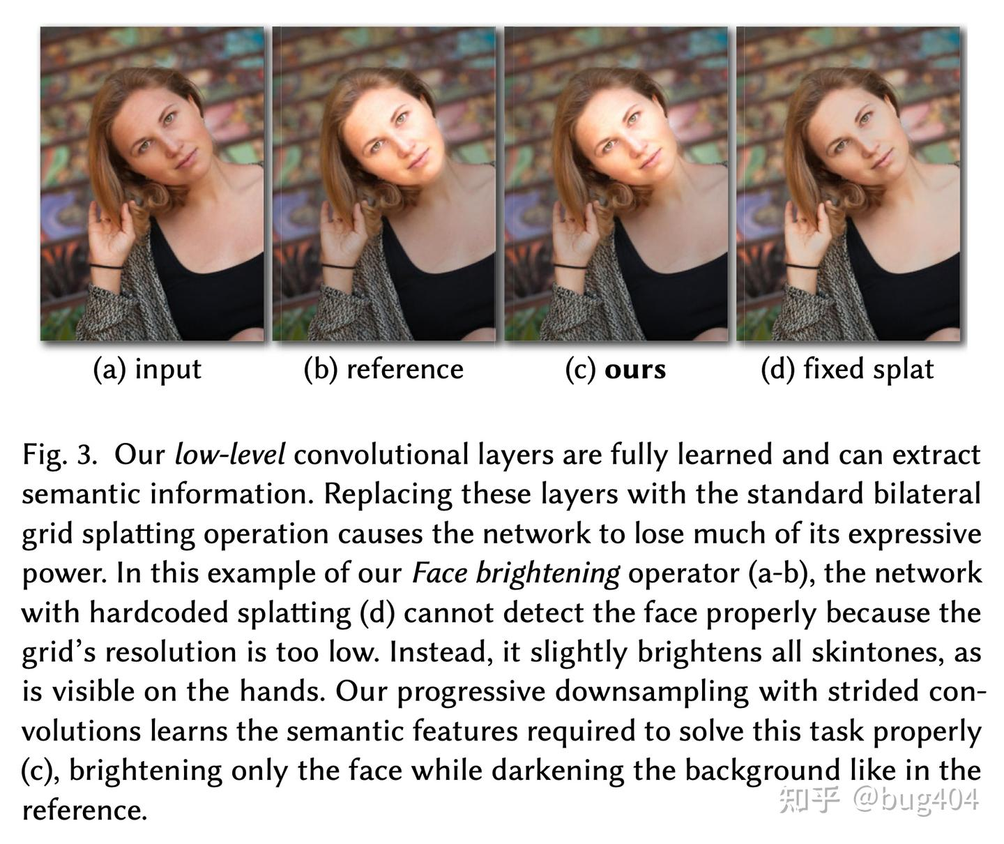
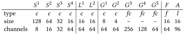
原图先通过下采样，得到256x256的固定大小，通过一系列卷积a stack of strided convolutional layers，得到low-level features之后。layer层数越多，下采样得到的图越小，low-level features的好处是最后的grid会更coarser，最后的特征图的感受野也越多，非线性更好，表达力更强。这其实就是CNN相比于手工设计特征的区别，可以准确地只对面部进行提亮：

# splat featuresn_layers_splat = int(np.log2(nsize/sb))self.splat_features = nn.ModuleList()prev_ch = 3for i in range(n_layers_splat):use_bn = bn if i > 0 else Falseself.splat_features.append(ConvBlock(prev_ch, cm*(2**i)*lb, 3, stride=2, batch_norm=use_bn))prev_ch = splat_ch = cm*(2**i)*lb

处理2D图像需要建立3D bilateral grid，可以把low res分支看作是learned splatting。

Since we produce a 3D bilateral grid from a 2D image in a content-dependent fashion, we can view the low-res stream as implementing a form of learned splatting.

得到low-level features之后，分为两部分：local和global

local

专注于提取local feature，使用fully convolutional，stride=1，特征图保持不变。这部分的 $n_L$ 和splat部分的 $n_S$ ，一共有 $n_S +n_L$ 层卷积。如果想要在更大的grid上计算coefficients，可以减少 $n_S$ ，但为了保持网络的表达能力，减少 $n_S$ 的同时要增大 $n_L$

# local featuresself.local_features = nn.ModuleList()self.local_features.append(ConvBlock(splat_ch, 8*cm*lb, 3, batch_norm=bn))self.local_features.append(ConvBlock(8*cm*lb, 8*cm*lb, 3, activation=None, use_bias=False))

global

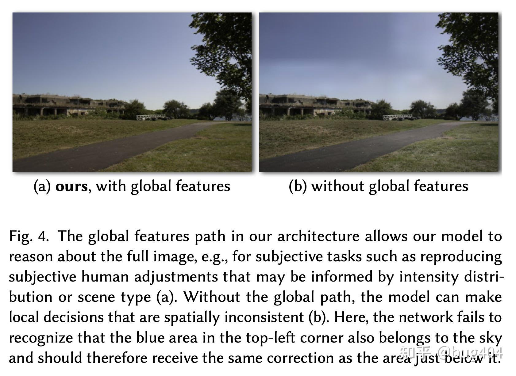
另外一路则同时使用2层stride=2的卷积和3层全连接，得到固定长度的全局信息fixed-size vector of global features，可以提取一些场景信息。使用全连接就意味着low-res input大小只能是固定大小，因为它的大小直接决定了全连接的参数量。但因为r slicing operator的存在，实际还是可以处理各种分辨率数据的。

# global featuresn_layers_global = int(np.log2(sb/4))self.global_features_conv = nn.ModuleList()self.global_features_fc = nn.ModuleList()for i in range(n_layers_global):self.global_features_conv.append(ConvBlock(prev_ch, cm*8*lb, 3, stride=2, batch_norm=bn))prev_ch = cm*8*lbn_total = n_layers_splat + n_layers_globalprev_ch = prev_ch * (nsize/2**n_total)**2self.global_features_fc.append(FC(prev_ch, 32*cm*lb, batch_norm=bn))self.global_features_fc.append(FC(32*cm*lb, 16*cm*lb, batch_norm=bn))self.global_features_fc.append(FC(16*cm*lb, 8*cm*lb, activation=None, batch_norm=bn))

全局特征分支得到64维的先验特征，用于指引局部特征，负责会出现一些不连续的artifacts：

The global path produces a 64-dimensional vector that summarizes global information about the input and acts as a prior to regularize the local decisions made by the local path.

fuse

融合使用了pointwise affine mixing，后面接Relu激活层。low_res_input=[H,W], 5层卷积之后的splat_feature [B,128,16,16], local feature尺寸(b,64,16,16)。这里的16就是spatial_bin。全局特征卷积之后的特征图尺寸是4，所以当spatial_bin=16的时候，全局特征使用两层卷积： $log_2 \frac{16}{4}$ 。

全局特征最后是(b,64)，长度和局部特征的通道数是一样的，view成(b,64,1,1)，这样local和gobal可以直接相加，相加之后使用1x1卷积，改变通道数，得到的通道数为lb*nout*nin，lb表示luma_bins=8，nin=4.nout=3,所以最后的通道数是96：

通道数为lb*nout*nin的x，使用torch.split以nout*nin为一组进行分组，得到tuple类型的tmp，之后再使用torch.stack对tmp进行合并，得到y，y相比于x，维度上升了一维。

把16x16x96拆分成了16x16x8x12，8就是bilateral grid中cell的个数，12表示的是4x3的仿射矩阵。

        fusion_grid = local_featuresfusion_global = global_features.view(bs,8*cm*lb,1,1)fusion = self.relu( fusion_grid + fusion_global )x = self.conv_out(fusion)s = x.shapey = torch.stack(torch.split(x, self.nin*self.nout, 1),2)# y = torch.stack(torch.split(y, self.nin, 1),3)

按照bilateral grid的思想应该是原始信号升维之后再进行滤波的，这里使用CNN在通道层面卷积之后再拆分开来，是殊途同归，这样就避免了三维卷积的使用。两种特征fuse得到的特征A（论文中的图2）可以看作是bilateral grid of affine coefficients

This operation is therefore more expressive than simply applying 3D convolutions in the grid, which would only induce local connectivity on z [Jampani et al. 2016]

.In a sense, by maintaining a 2D convolution formulation throughout and only interpreting the last layer as a bilateral grid, we let the network decide when the 2D to 3D transition is optimal.

guide

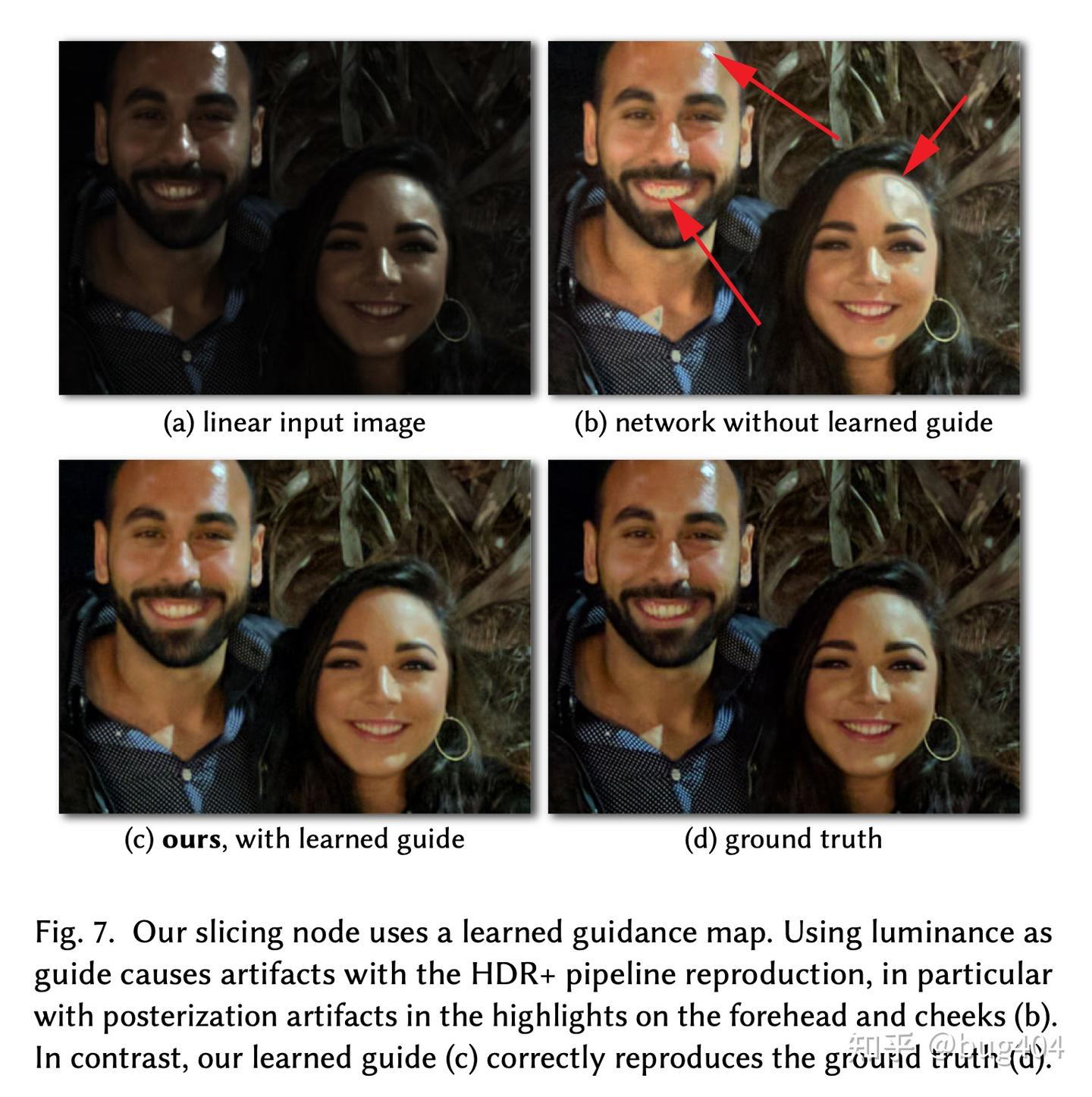
对全尺寸高分辨率图进行处理。stride=1，padding=0，结果两层卷积之后分辨率没用发生变化。得到的guide map是一个单通道的图。

这里的特征提取也是很重要的，下面的结果就表明了learned guide比亮度作为引导图，有更好的效果：

slice

二维图像得到的grid是3D的，分别是x，y，val：

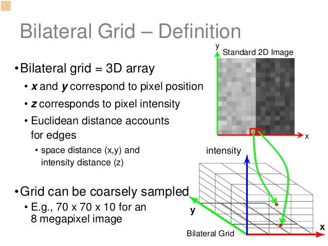
3D grid通过升维把空间信息和像素值信息放在了同一个空间下，是bilateral grid思想的延续。为了进一步减少计算量，grid相比于guide可以是尺寸更小的。上图中就提到，70x70x10的grid可以对应800万像素的图像。

如fuse章节所说，具体实现时使用的仍然是2D卷积，只不过把c通道进行了重新划分。所以最终grid是5维的[B,in*out,n,H,W],permute之后是[B,H,W,n,in*out]，B是batchsize，n表示对guide的量化级数，in*out表示每个cell的变换系数。

对batch中的每个样本做处理。slice的输入是guide map g 和feature map A (viewed as a bilateral grid)，输出是a new feature map，但是分辨率和guide map g一样，所以slice本质是一个上采样的过程，使用的是 tri-linearly interpolating

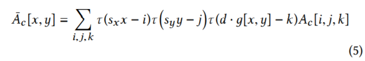
x,y经过比例映射到grid的位置，与i，j越近，权重会越大。亮度g则是经放大d倍后与k相比，越相近权重越大。这里的d=8，意味着亮度只分了8个级别。

这个过程没用参数需要学习，所以可以使用OpenGL实现。因为有guide map的使用，相比于反卷积，有更好的边缘恢复。

applay_coeffs

局部看作是仿射变换

recent work has observed that even complicated image processing pipelines can often be accurately modeled as a collection of simple local transformations [Chen et al. 2016; Gharbi et al. 2015; He and Sun 2015].

所以原始rgb经过3x4大小的矩阵映射就得到了输出：

        '''Affine:r = a11*r + a12*g + a13*b + a14g = a21*r + a22*g + a23*b + a24...'''R = torch.sum(full_res_input * coeff[:, 0:3, :, :], dim=1, keepdim=True) + coeff[:, 9:10, :, :]G = torch.sum(full_res_input * coeff[:, 3:6, :, :], dim=1, keepdim=True) + coeff[:, 10:11, :, :]B = torch.sum(full_res_input * coeff[:, 6:9, :, :], dim=1, keepdim=True) + coeff[:, 11:12, :, :]return torch.cat([R, G, B], dim=1)

reference：

1.https://zhuanlan.zhihu.com/p/587350063

2.https://zhuanlan.zhihu.com/p/37404280

3.https://zhuanlan.zhihu.com/p/614185346

4.https://groups.csail.mit.edu/graphics/hdrnet/data/hdrnet.pdf

5.https://zhuanlan.zhihu.com/p/37404280

6.https://zhuanlan.zhihu.com/p/614185346

7.https://zhuanlan.zhihu.com/p/537612591

查看全文

http://www.xdnf.cn/news/2139.html