怎样用 esProc 实现多数据库表的数据合并运算
由于业务需要将数据按年存储在两个结构相同的数据库中,要进行数据统计就会涉及多库混合计算。通过数据库或硬编码实现都比较麻烦,借助 esProc 可以简化这类运算。
数据
orders 表结构:
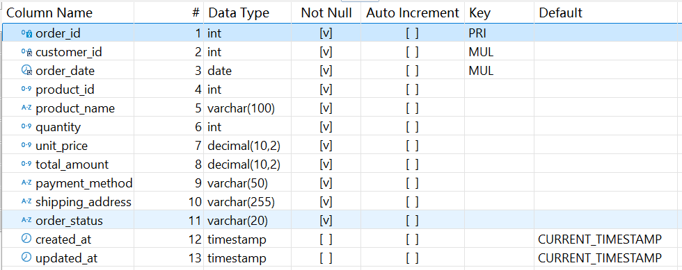
其中 order_id 是主键。
数据样例:
10001	16	2024-12-14	116	Product116	9	12.84	115.56	Credit Card	984 Example St, City 2	Pending	2025-04-23 01:21:08	2025-04-23 01:21:08
10002	11	2024-08-18	116	Product116	5	25.71	128.55	PayPal	841 Example St, City 1	Shipped	2025-04-23 01:21:08	2025-04-23 01:21:08
10003	20	2024-08-08	109	Product109	2	13.23	26.46	PayPal	676 Example St, City 4	Pending	2025-04-23 01:21:08	2025-04-23 01:21:08
10127	7	2024-10-12	113	Product113	4	20.64	82.56	Cash	145 Example St, City 4	Delivered	2025-04-23 01:21:08	2025-04-23 01:21:08
10190	19	2024-06-02	110	Product110	7	88.55	619.85	PayPal	289 Example St, City 2	Pending	2025-04-23 01:21:08	2025-04-23 01:21:08
现在要合并计算两个库的数据。用 esProc 怎么做呢?
安装 esProc
先通过下载免费的esProc SPL 选择esProc 标准版。
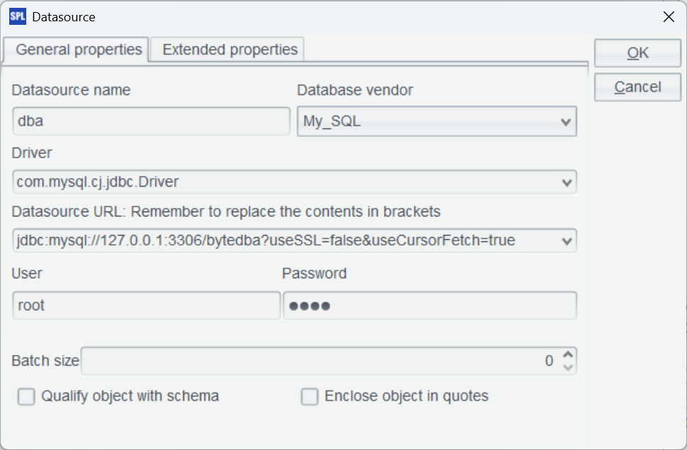
安装后,配 MySQL 数据库连接。
先把 MySQL JDBC 驱动包放到 [esProc 安装目录]\common\jdbc 目录下(其他数据库类似)。
然后启动 esProc IDE,菜单栏选择 Tool-Connect to Data Source,配置 MySQL 标准 JDBC 连接。
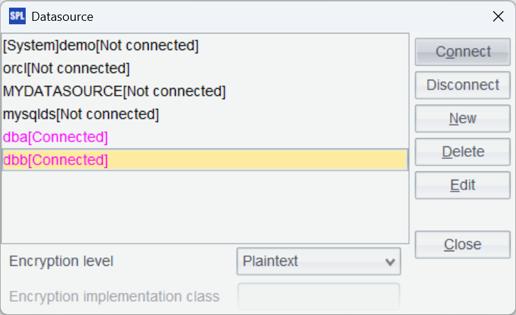
同样的方式配置 bytedbb 库的数据源 dbb。测试一下连接,点击 Connect,发现刚刚配置的两个数据源变成粉红色证明连接成功。
测试一下,按 ctrl+F9 执行脚本,可以正常查询数据说明配置没问题
混算
下面把两个表的数据合并一起计算。
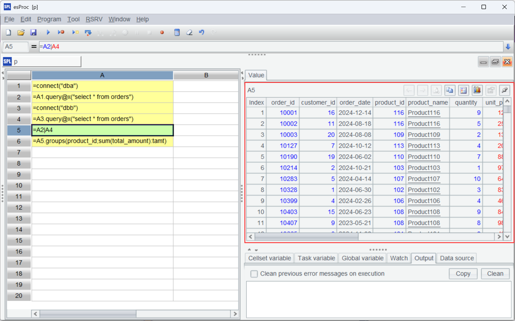
| A | |
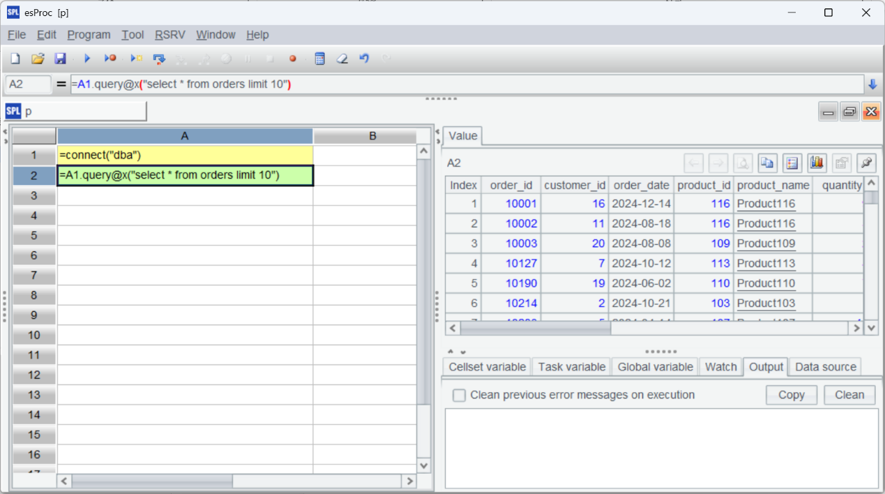
| 1 | =connect("dba") |
| 2 | =A1.query@x("select * from orders") |
| 3 | =connect("dbb") |
| 4 | =A3.query@x("select * from orders") |
| 5 | =A2|A4 |
| 6 | =A5.groups(product_id;sum(total_amount):tamt) |
A2 和 A4 分别查询两个库的 orders 数据,@x 选项表示查询后关闭连接。A5 使用“|”符号合并两部分数据,就这么简单。然后 A6 基于合并结果进行后续计算(这里是分组汇总)。
点击某个单元格(如合并数据的 A5),可以看到该步骤的计算结果。
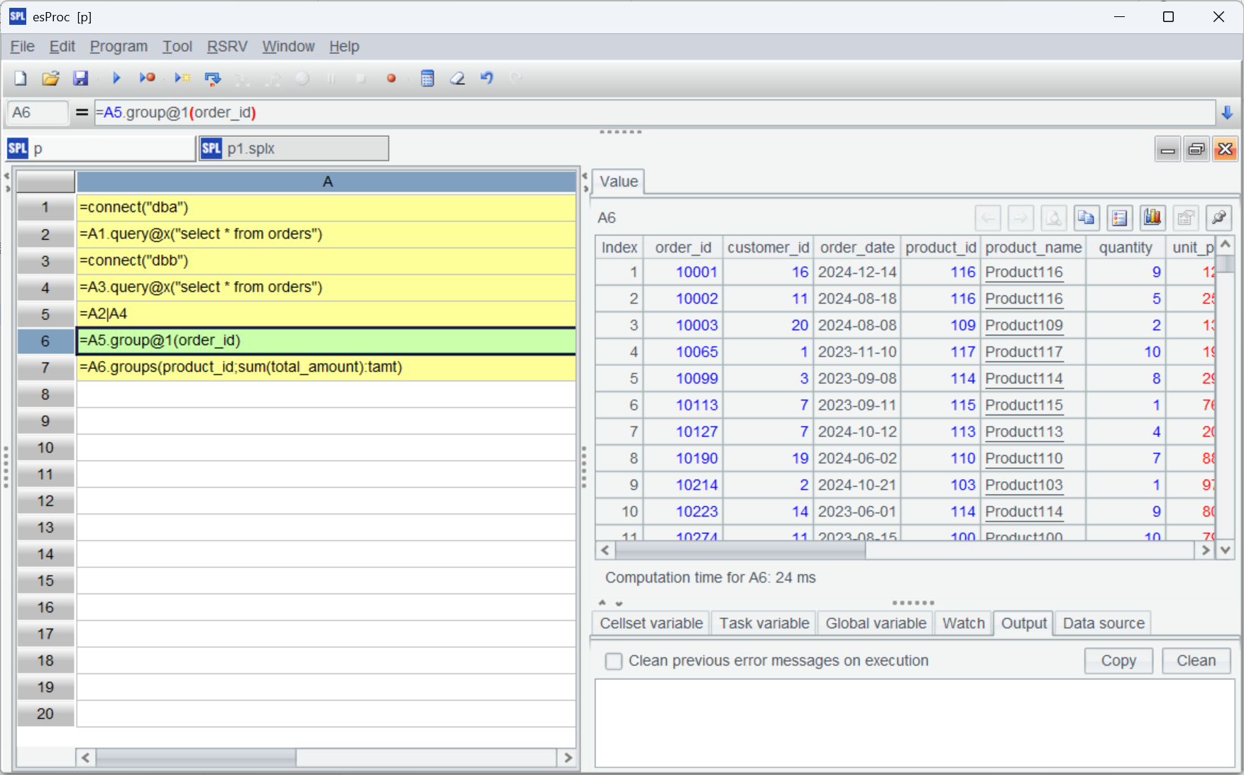
但是我们发现两个库的数据有重复,需要去重后再计算。
| A | |
| 1 | =connect("dba") |
| 2 | =A1.query@x("select * from orders") |
| 3 | =connect("dbb") |
| 4 | =A3.query@x("select * from orders") |
| 5 | =A2|A4 |
| 6 | =A5.group@1(order_id) |
| 7 | =A6.groups(product_id;sum(total_amount):tamt) |
A6 使用 group@1 对 order_id 分组且只保留分组中的第一条记录,这样就去除了重复。如果想根据条件保留记录(比如时间最近的),就可以先排序再 group@1,很灵活。
查看 A6 的结果,发现原来两表中都包含 id 是 10001,10002 等重复数据都去除了,A7 再进行分组汇总。
后续的计算仍然跟单表一样,如果想做其他计算只需要换个计算表达式就可以。
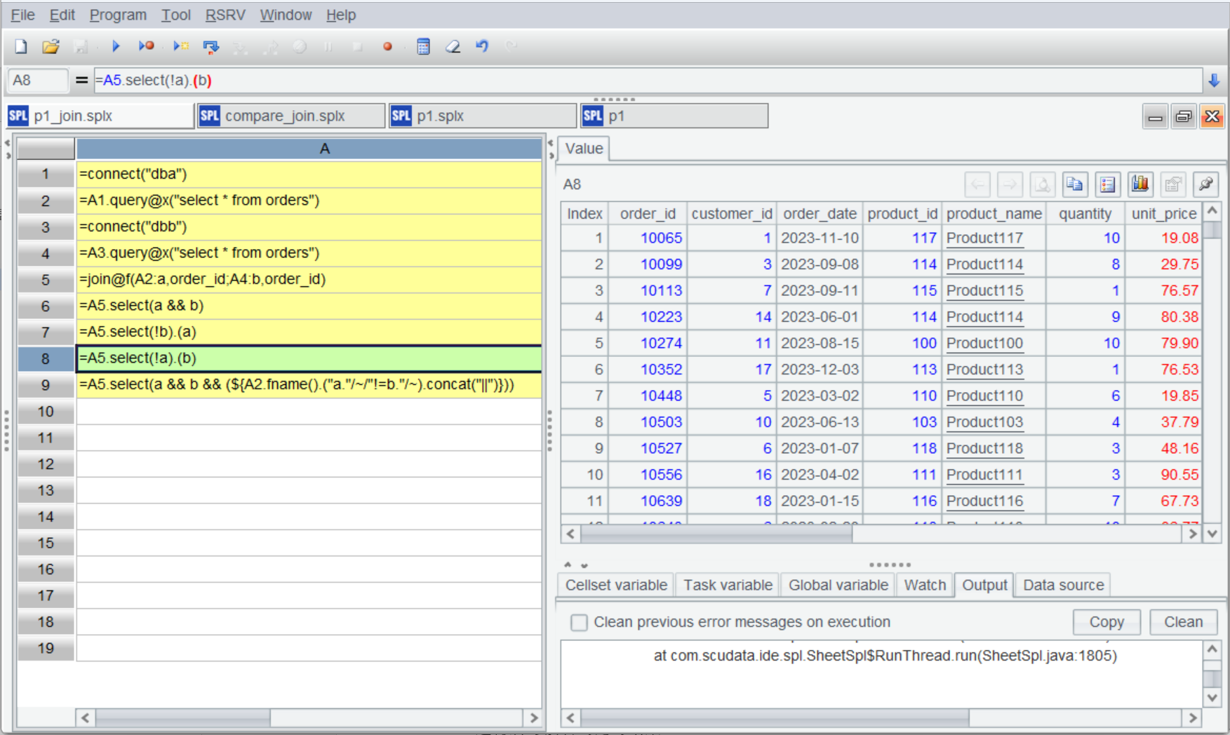
能做混合计算,也就能顺便解决数据比对任务。比如查找两库都有的订单、仅存在一个库的订单等。
| A | |
| 1 | =connect("dba") |
| 2 | =A1.query@x("select * from orders") |
| 3 | =connect("dbb") |
| 4 | =A3.query@x("select * from orders") |
| 5 | =join@f(A2:a,order_id;A4:b,order_id) |
| 6 | =A5.select(a && b) |
| 7 | =A5.select(!b).(a) |
| 8 | =A5.select(!a).(b) |
| 9 | =A5.select(a && b && (${A2.fname().("a."/~/"!=b."/~).concat("||")})) |
这里 A5 使用 join 做全连接,A6 筛选重复订单(交集),A7 和 A8 分别筛选不重复订单(差集),A9 筛选 order_id 重复但其他列不同的记录,这里用到宏来简化书写,${A2.fname().("~(1)."/~/"!=~(2)."/~).concat("||") 展开后是这样:~(1).quantity != ~(2).quantity || ~(1).unit_price != ~(2).unit_price || ~(1).total_amount != ~(2).total_amount || ~(1).order_status != ~(2).order_status
运行后可以看到比对结果:
大数据情况
如果数据量比较大不能把数据全部读入内存,就需要使用 esProc 的游标机制完成混合计算。
如果不需要去重,简单把把两个游标合并到一起计算就行:
| A | |
| 1 | =connect("dba") |
| 2 | =A1.cursor@x("select * from orders") |
| 3 | =connect("dbb") |
| 4 | =A3.cursor@x("select * from orders") |
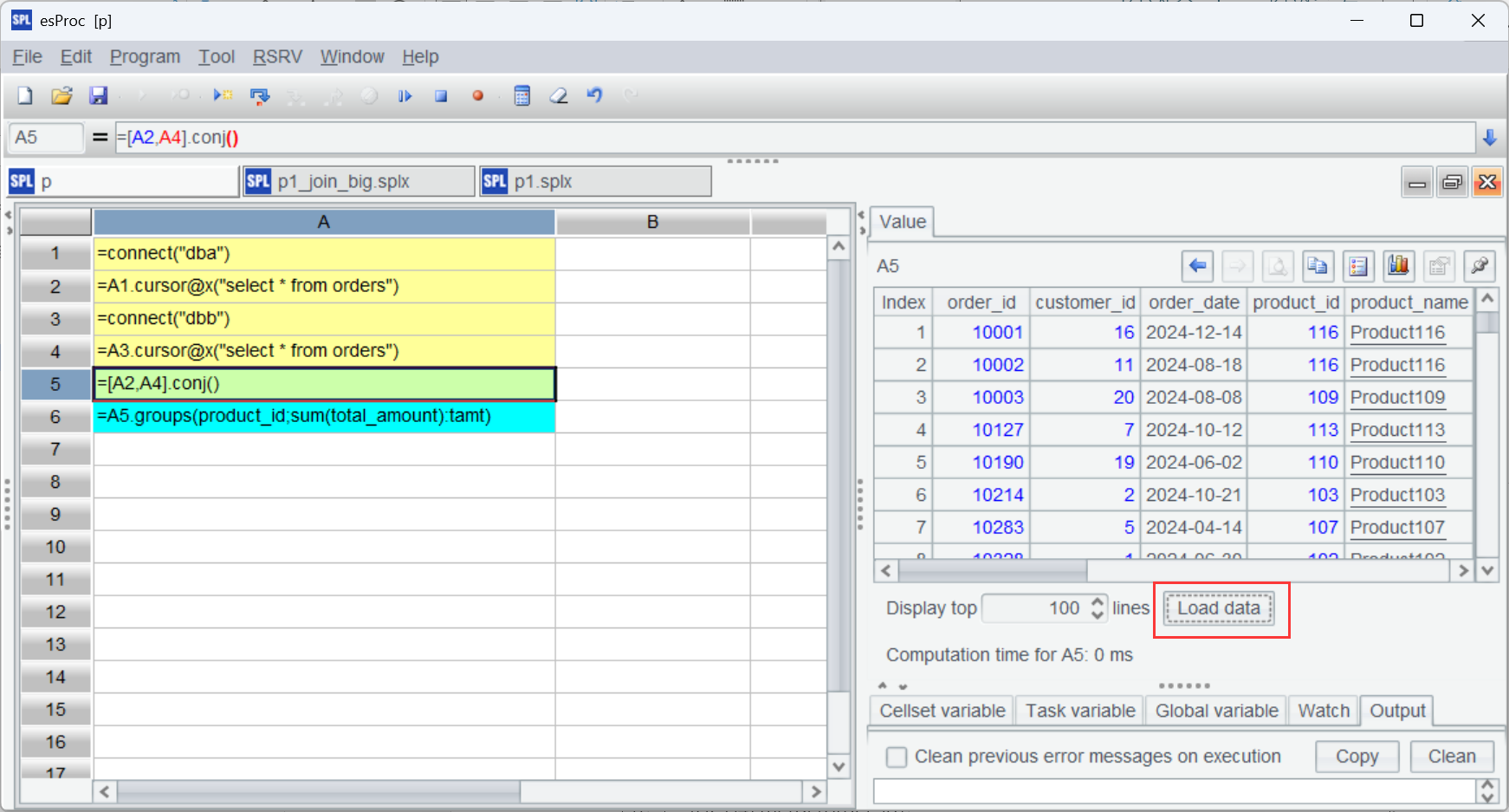
| 5 | =[A2,A4].conj() |
| 6 | =A5.groups(product_id;sum(total_amount):tamt) |
A2 和 A4 使用 cursor 函数查询数据,在 A5 中合并两个游标,在 A6 进行计算。整体跟全内存计算差别不大。
执行脚本, A5 返回的是游标对象,如果想查看里面的内容可以点击“load data”:
如果要先做去重,需要游标保持有序才能方便比较相邻数据。这里要在 SQL 中按 order_id 排序。
| A | |
| 1 | =connect("dba") |
| 2 | =A1.cursor@x("select * from orders") |
| 3 | =connect("dbb") |
| 4 | =A3.cursor@x("select * from orders") |
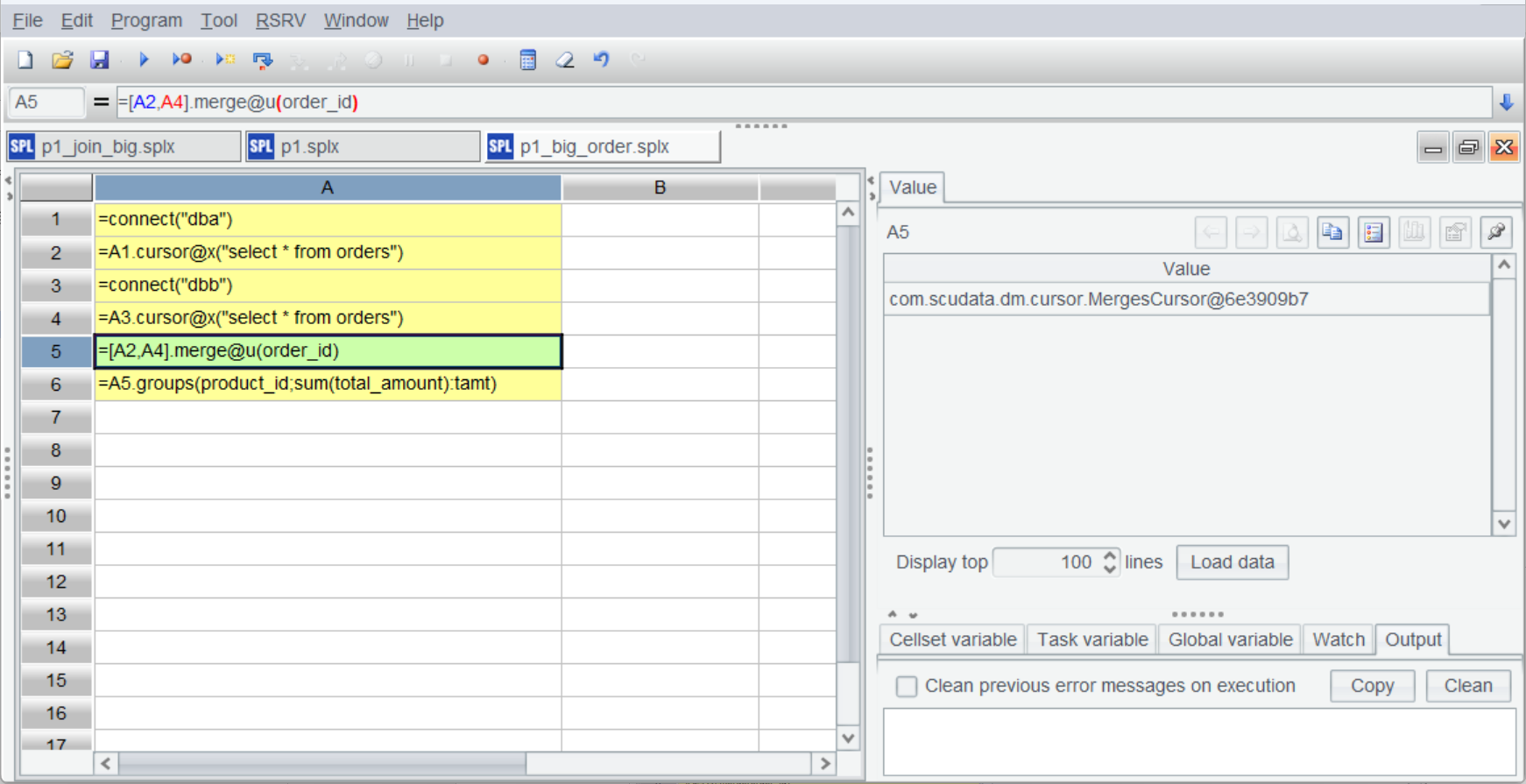
| 5 | =[A2,A4].merge@u(order_id) |
| 6 | =A5.groups(product_id;sum(total_amount):tamt) |
归并有序游标需要使用 CS.merge() 函数,merge 提供了很多选项,@u 表示求并集,所以直接就去重了。还有 @i 表示交集,@d 表示差集。后续的计算就都一样了。
Merge 后返回的仍是游标(并不进行实质的计算):
执行到最后的分组汇总才开始计算并返回结果。
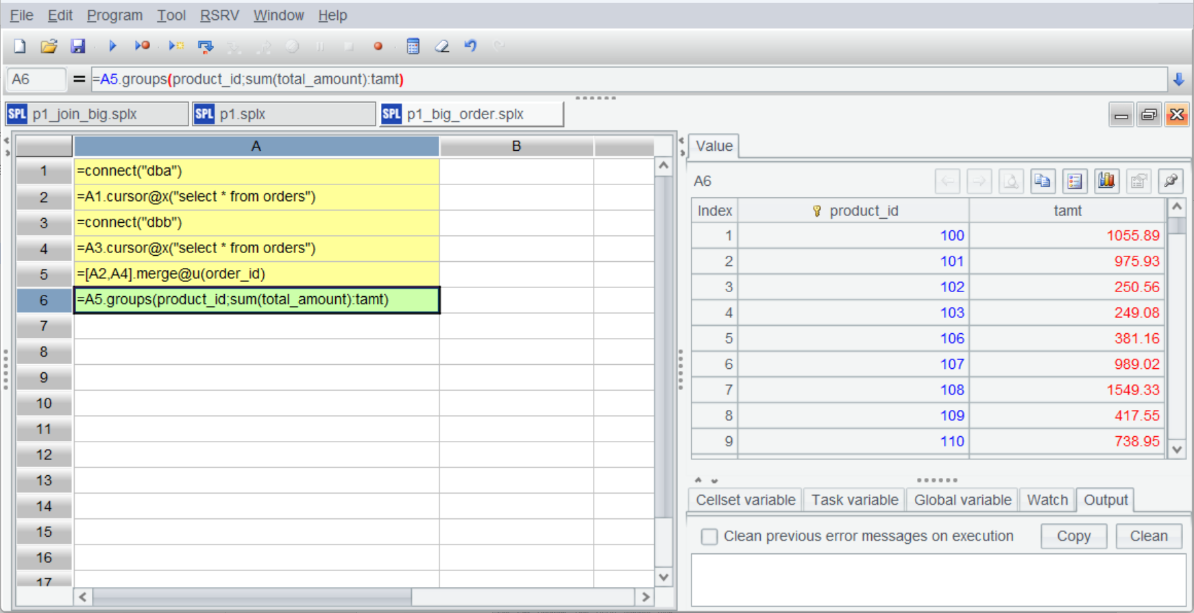
整体上大数据情况的计算过程与全内存时基本一致,可以有效降低使用门槛。
大数据的比对也可以做:
| A | B | |
| 1 | =connect("dba") | |
| 2 | =A1.query("select column_name from information_schema.columns where table_schema ='bytedba'and table_name ='orders'") | |
| 3 | =A1.cursor@x("select * from orders order by 1") | |
| 4 | =connect("dbb") | |
| 5 | =A4.cursor@x("select * from orders order by 1") | |
| 6 | =joinx@f(A3:a,order_id;A5:b,order_id) | |
| 7 | =A6.select(a && b) | =A7.fetch() |
| 8 | =A6.select(!b).(a) | =A8.fetch() |
| 9 | =A6.select(!a).(b) | =A9.fetch() |
| 10 | =A5.select(a && b && (${A2.(#1).("a."/~/"!=b."/~).concat("||")})) | =A10.fetch() |
由于 A6-A10 返回的都是游标,所以需要在 B7-B10 上增加结果集函数来执行计算并获取结果。
但奇怪的是只有 B7 有结果,B8-B10 都是空的。
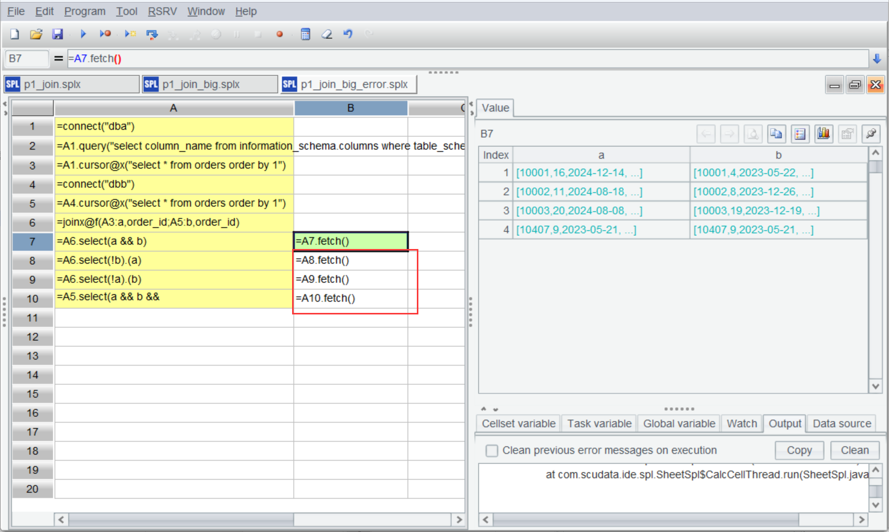
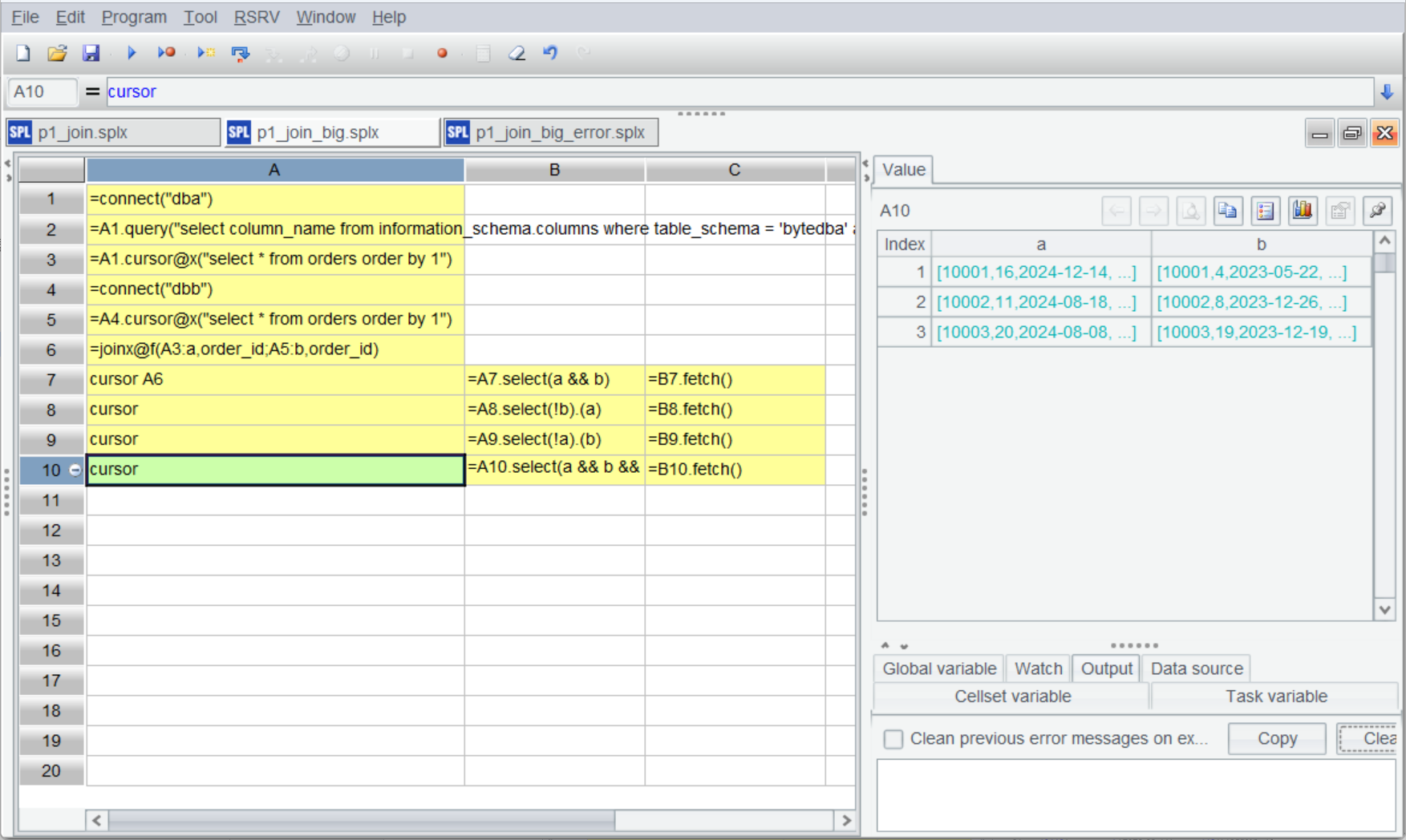
这是因为游标是一次性的,一次遍历完就结束了,后面的计算也就没法再进行了。这时就要借助 esProc 提供的游标复用(管道)机制,大数据情况下一次遍历完成多个计算。我们来改造一下代码:
| A | B | C | |
| 1 | =connect("dba") | ||
| 2 | =A1.query("select column_name from information_schema.columns where table_schema ='bytedba'and table_name ='orders'") | ||
| 3 | =A1.cursor@x("select * from orders order by 1") | ||
| 4 | =connect("dbb") | ||
| 5 | =A4.cursor@x("select * from orders order by 1") | ||
| 6 | =joinx@f(A3:a,order_id;A5:b,order_id) | ||
| 7 | cursor A6 | =A7.select(a && b) | =B7.fetch() |
| 8 | cursor | =A8.select(!b).(a) | =B8.fetch() |
| 9 | cursor | =A9.select(!a).(b) | =B9.fetch() |
| 10 | cursor | =A10.select(a && b && (${A2.(#1).("a."/~/"!=b."/~).concat("||")})) | =B10.fetch() |
A7-A10 基于 A5 的游标创建管道(A8-A10 是省略写法),剩下 B7-C10 的运算跟上面就完全一样了。运行后我们可以在 A7-A10(注意不是 C7-C10)格看到计算后的结果。
如果计算结果也比较大没法全内存,还可以将结果输出到文件。再改造一下上面的代码:
| A | B | C | |
| 1 | =connect("dba") | ||
| 2 | =A1.query("select column_name from information_schema.columns where table_schema ='bytedba'and table_name ='orders'") | ||
| 3 | =A1.cursor@x("select * from orders order by 1") | ||
| 4 | =connect("dbb") | ||
| 5 | =A4.cursor@x("select * from orders order by 1") | ||
| 6 | =joinx@f(A3:a,order_id;A5:b,order_id) | ||
| 7 | cursor A6 | =A7.select(a && b) | >B7.fetch("intersec.btx") |
| 8 | cursor | =A8.select(!b).(a) | >B8.fetch("diff_a.btx") |
| 9 | cursor | =A9.select(!a).(b) | >B9.fetch("diff_b.btx") |
| 10 | cursor | =A10.select(a && b && (${A2.(#1).("a."/~/"!=b."/~).concat("||")})) | >B10.fetch("comp.btx") |
在 C7-C10 的 fetch 中加入输出文件名。
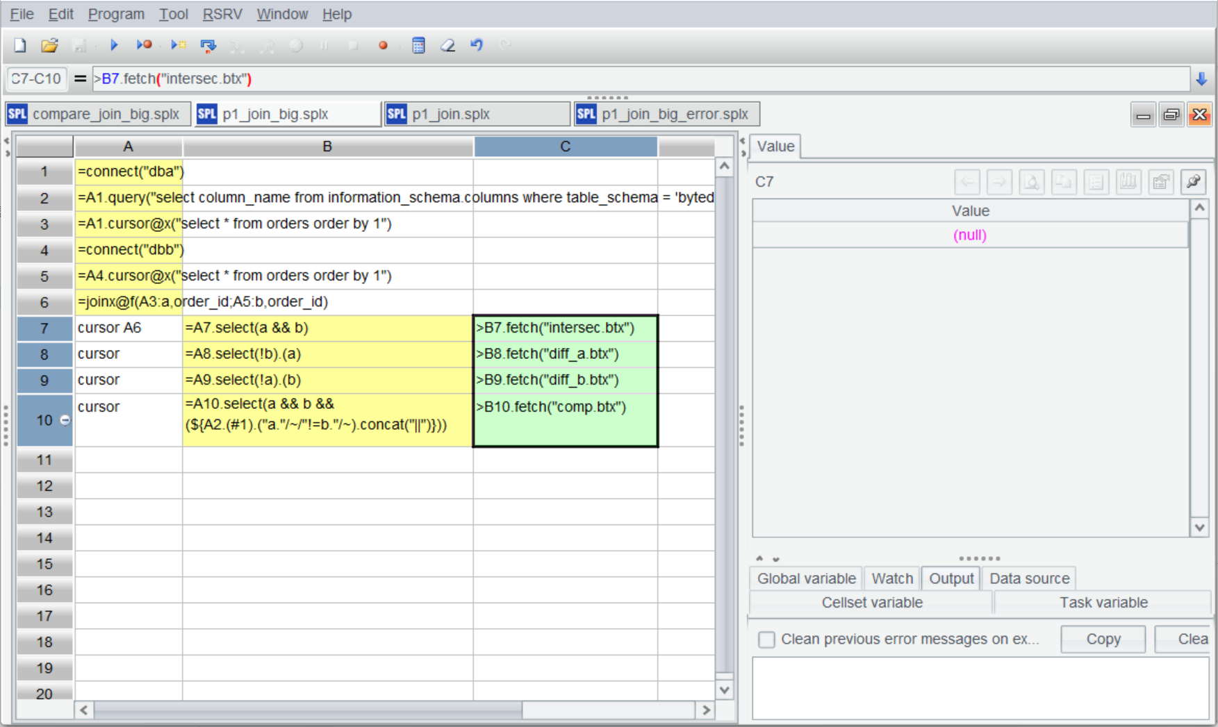
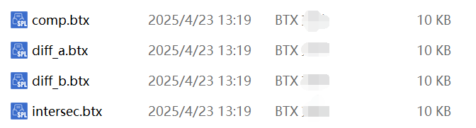
执行后就得到了这几个结果文件。
涉及跨库的混合计算用 esProc 就都能搞定了。
esProc 脚本可以很方便地嵌入到 Java 应用中,部署集成步骤可参考乾学院的文档。